Hierarchy between forelimb premotor and primary motor cortices and its manifestation in their firing patterns
- Department of Neurobiology, Northwestern University, United States
Figures
Figure 1 with 1 supplement
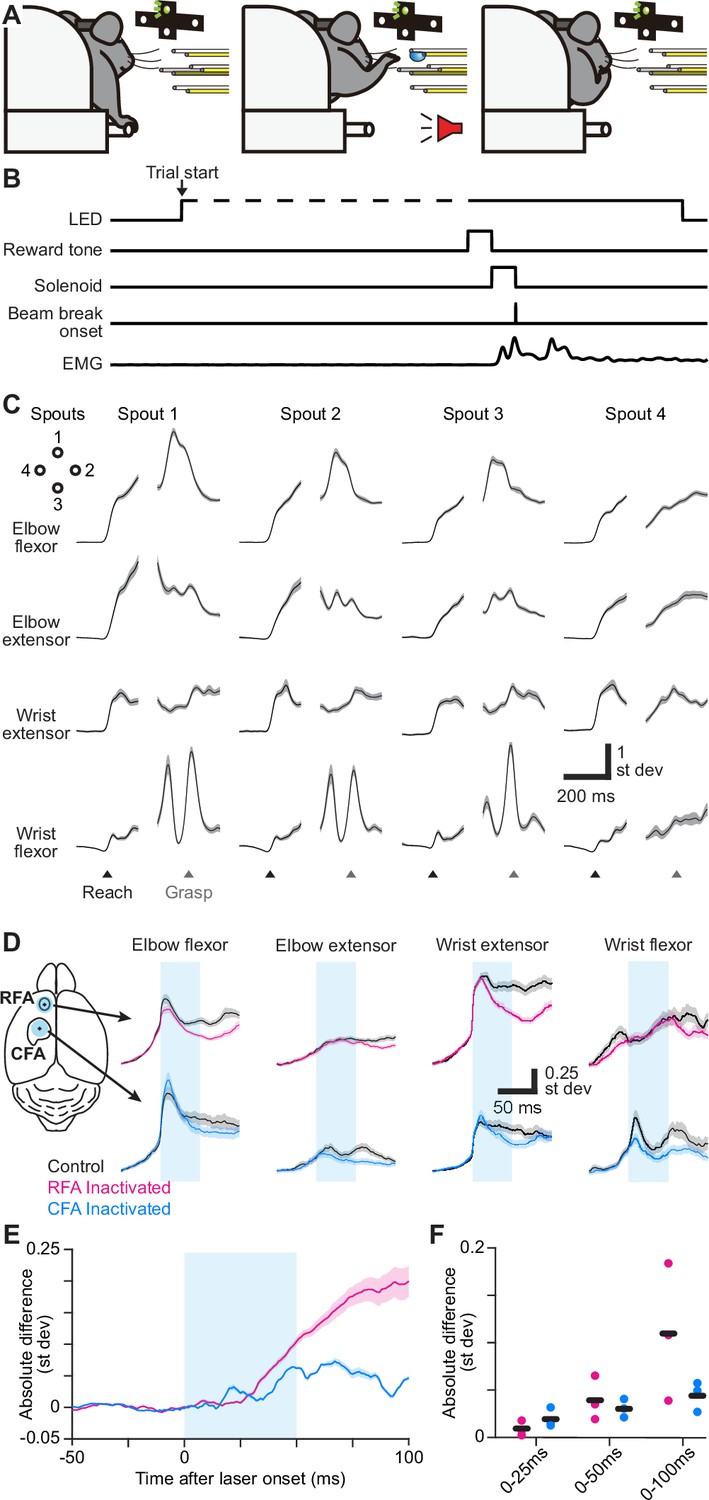
RFA and CFA influence on forelimb muscles during directional reaching in mice.
(A) Schematic depicting the directional reaching task. (B) Schematic depicting the time course of experimental control signals and muscle activity during the directional reaching task. (C) Trial-averaged activity of four recorded muscles (black) ± SEM (gray, n=176 trials) for one mouse during directional reaching toward each of four spouts. Separate averages are aligned on reach onset (Reach) or spout contact (Grasp). Vertical scale bars in (C) and (D) reflect standard deviation of z-scored muscle activity. (D) For one example mouse, mean ± SEM muscle activity for trials without (black) or with inactivation (50ms, cyan bar) of RFA (top, magenta) or CFA (bottom, blue) triggered on reach onset. Left image shows the position of the light stimulus on RFA and CFA. (E) Mean ± SEM absolute difference between inactivation and control trial averages across all recorded muscles (n=12 from 3 animals) for inactivation (50ms, cyan bar) of RFA or CFA. For baseline subtraction, control trials were resampled to estimate the baseline difference expected by chance. This subtraction leads to values below zero. (F) Absolute difference between inactivation and control trials averaged over three epochs after light/trial onset, for individual animals (circles) and the mean across animals (black bars).
Figure 1—figure supplement 1

Extended time series from Figure F1D.
For one example mouse, mean ± SEM muscle activity for trials without (black) or with inactivation (50ms, cyan bar) of RFA (top, magenta) or CFA (bottom, blue) triggered on reach onset. Left image shows the position of the light stimulus on RFA and CFA.
Figure 2 with 1 supplement
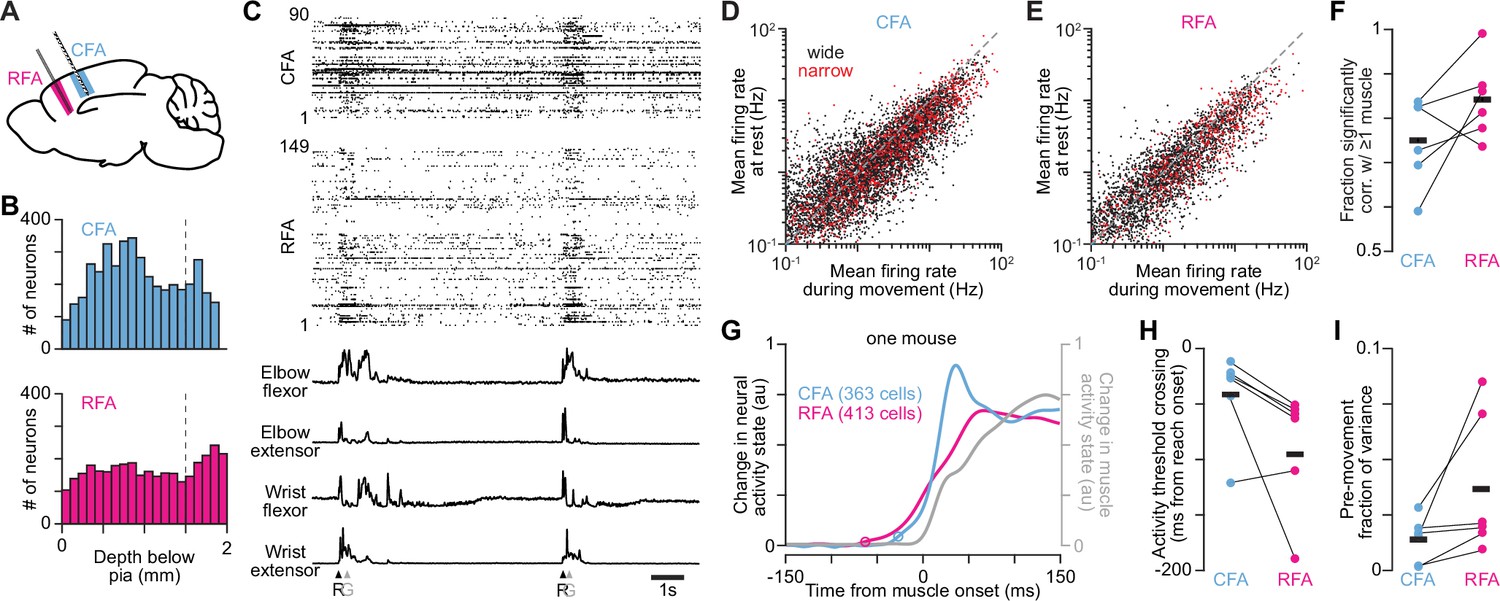
RFA and CFA activity during directional reaching in mice.
(A) Mouse brain schematic depicting recordings in RFA and CFA. (B) Histograms showing the depth below pia of single unit isolations (neurons) recorded with Neuropixels and extracted with Kilosort. Dotted vertical lines depict where the cutoff for the bottom of each cortical region was defined. (C) Example of spike rasters (top) and muscle activity (bottom) recorded in one mouse during reach performance. Arrowheads indicate each onset (R) or spout contact (G). (D), (E) Scatter plots of the firing rates for neurons recorded in CFA (D) and RFA (E) during epochs when mice are activating their forelimb muscles, versus periods when all muscles are quiescent, separated for neurons that have wide and narrow waveforms. (F) The fractions of neurons recorded in both CFA and RFA whose firing rate time series was significantly correlated with that of at least one muscle (p-value threshold = 0.05), for individual animals (circles) and the mean across animals (black bars, n=6 mice). (G) For one mouse, normalized absolute activity change from baseline summed across the top three principal components (PCs) for all recorded RFA or CFA neurons, and the top PC for muscle activity. Circles indicate the time of detected activity onset. The pre-reach baseline epoch was from 150 ms to 100 ms before reach onset. Neural activity onset was detected as the first time at which activity rose 11 standard deviations above baseline. (H) Time from reach onset at which the activity change from baseline summed across the top PCs for RFA (magenta) or CFA (blue) neurons rose above a low threshold, for individual animals (circles) and the mean across animals (black bars, n=6 mice). (I) The activity variance in the 150ms before muscle activity onset, defined as a fraction of the total activity variance from 150ms before to 150ms after muscle activity onset, for each animal (circles) and the mean across animals (black bars, n=6 mice).
Figure 2—figure supplement 1
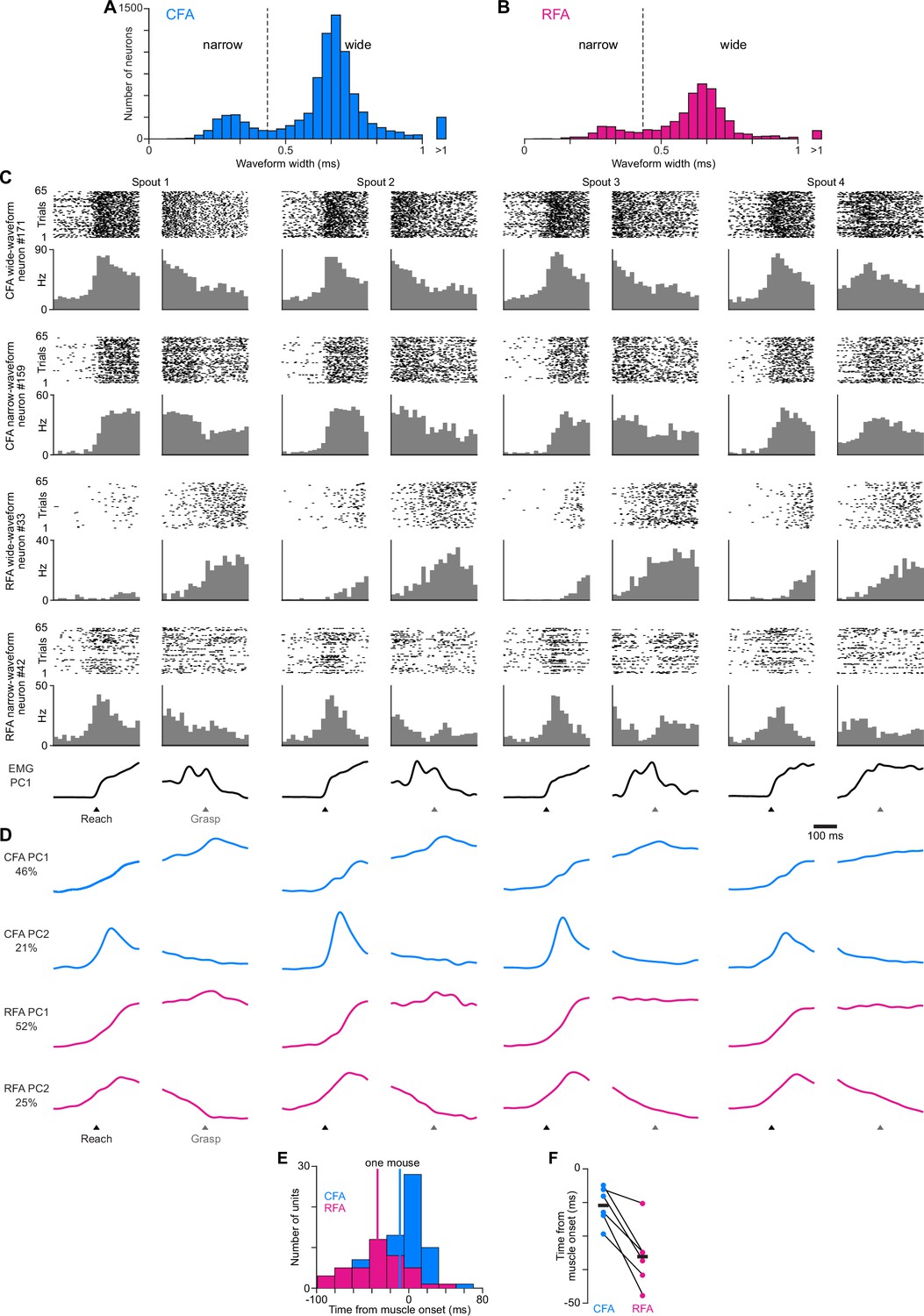
RFA and CFA activity during directional reaching in mice.
(A), (B) Histograms of waveform widths for recorded neurons in CFA (A) and RFA (B), showing the bimodal distribution of narrow and wide waveforms. Dotted line shows the threshold above which neurons were considered wide waveform. (C) For four example neurons, spike rasters (top) and binned firing rate (bottom) across all successful reach trials to each spout, aligned on reach onset (black arrowheads) and spout contact (Grasp, gray arrowheads). Bottom row shows the corresponding time series for the first principal component of muscle activity. (D) CFA (blue) and RFA (magenta) activity projected onto their respective first two principal components, from the recording involving the neurons shown in (A). (E) For one mouse, a histogram of the time around reach onset when the firing rate of individual neurons rises above a pre-reach baseline, for RFA or CFA neurons. Vertical lines indicate the mean across neurons for each region. To avoid neurons with noisy mean firing rates, the analysis depicted in (E), (F) included only the neurons with mean firing rates above the 90th percentile value for each given animal. Onset time for each neuron was detected by finding the time at which its trial-averaged firing rate first rose above a threshold defined as 7 standard deviations above the mean for a pre-reach baseline epoch (150 ms to 100 ms before reach onset). (F) Mean time from reach onset at which the firing rate of individual neurons rises above a pre-reach baseline for RFA or CFA neurons, for individual animals (circles) and the mean across animals (black bars, n=6 mice).
Figure 3 with 1 supplement
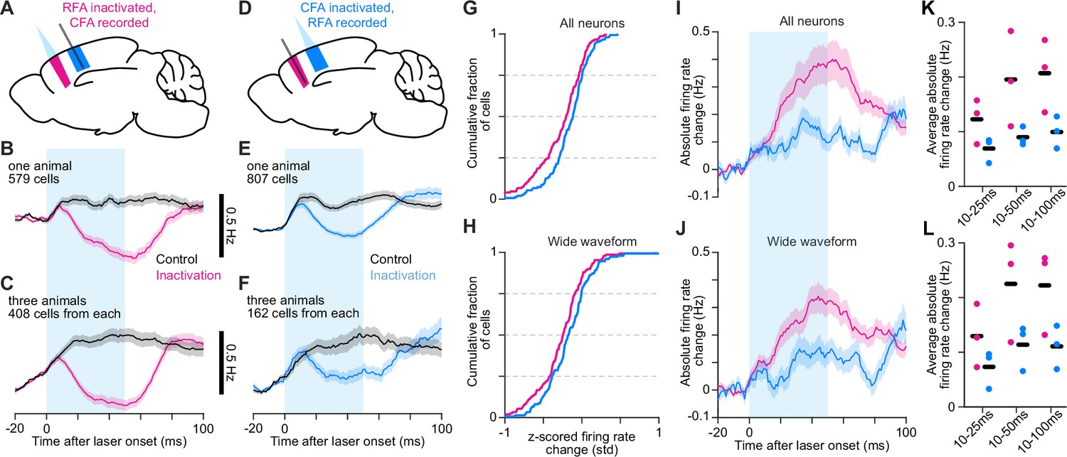
Asymmetric reciprocal influence of endogenous RFA and CFA activity.
(A–F) Schematics depicting inactivation and Neuropixel recording (A,D) and mean ± SEM firing rate time series for neurons from one animal (B,E) or all three animals (C,F) from inactivating RFA and recording CFA (A–C), or vice versa (D–F). The cyan bar indicates light on. The same number of cells was used from each animal in (C) and (F). The minimum firing rates for the inactivation trial averages are as follows: (B) 0.72 Hz, (C) 1.18 Hz, (E) 0.42 Hz, (F) 0.89 Hz. (G), (H) Cumulative histograms of the difference between averaged z-scored firing rates for control and inactivation trials averaged from 45 to 55ms after light/trial onset, for the top 50 highest firing rate neurons (G) or wide-waveform neurons (H) from each animal, combined. (I), (J) Mean absolute firing rate difference ± SEM between control and inactivation trial averages for all (I) and wide-waveform (J) neurons recorded in the other area during RFA and CFA inactivation. The same number of cells was used from each animal. Baseline subtraction enables negative values. (K), (L) Average absolute firing rate difference from 10ms after light onset to 25, 50, and 100ms after for all (K) and wide-waveform (L) neurons, for individual animals (circles) and the mean across animals (black bars).
Figure 3—figure supplement 1
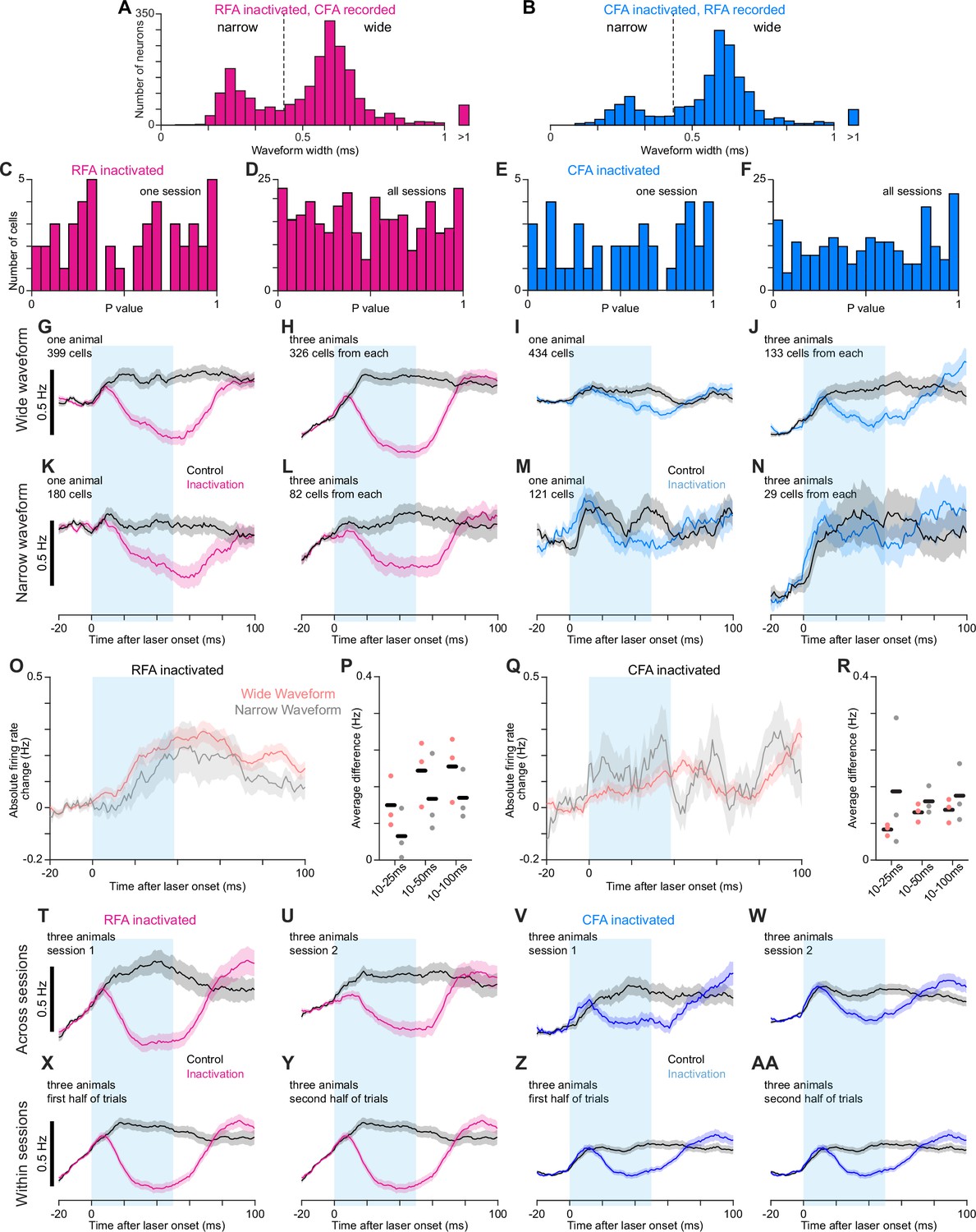
Effects of CFA and RFA inactivation on firing rates in the other region.
(A), (B) Histograms of waveform widths for recorded neurons in CFA (A) and RFA (B), showing the bimodal distribution of narrow and wide waveforms. Dotted line shows the threshold above which neurons were considered wide waveform. (C)-(F) Histograms of p-values from our modified version of SALT for narrow-waveform neurons recorded in one session (C,E) or all sessions (D,F) in either CFA (C,D) or RFA (E,F) while inactivating the other region. The uniformity of these distributions indicates an absence of appreciable violation of the null hypotheses that neurons are not directly activated by light. (G)-(N) Mean firing rate ± SEM for wide-waveform (G–J) or narrow-waveform (K–N) neurons for one animal (G,I,K,M) or three animals (H,J,L,N) recorded in CFA (G,H,K,L) or RFA (I,J,M,N) while inactivating the other region. Averages combining cells from multiple animals used the same number of cells from each animal. The cyan rectangle indicates when the light was applied. (O)-(R) Mean absolute firing rate change ± SEM between control and inactivation trials (O,Q) and mean absolute firing rate difference between control and inactivation trials averaged from 10ms after light/trial onset to 25, 50, or 100ms afterwards (P,R) for wide- and narrow-waveform neurons recorded in CFA (O,P) or RFA (Q,R) during inactivation of the other region. Black bars show mean across animals. (T)-(AA) Mean firing rate ± SEM for all three animals recorded in CFA (T,U,X,Y) or RFA (V,W,Z,AA) while inactivating the other region, either for two separate sessions (T–W) or the first and second half of trials from all sessions (X–AA). The cyan rectangle indicates when the light was applied. Average inactivation effects show remarkable consistency, both within and across sessions.
Figure 4 with 1 supplement
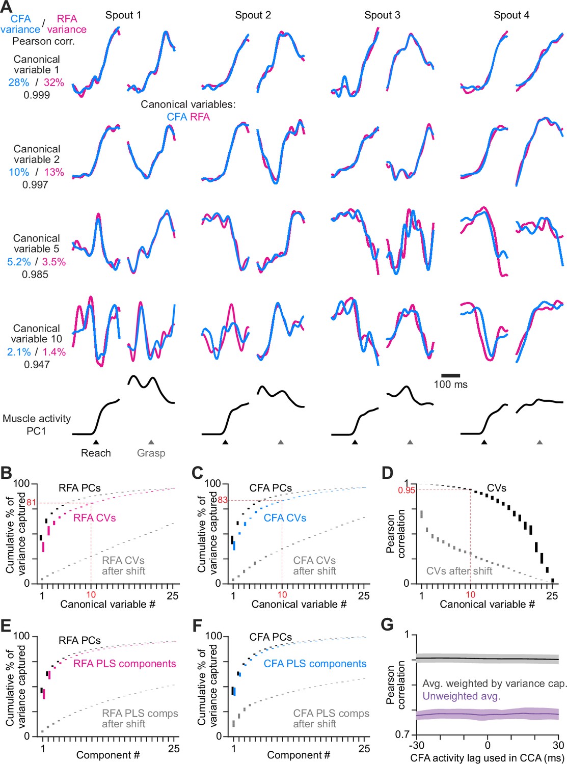
RFA and CFA firing patterns during reaching are highly similar.
(A) From one animal, four canonical variables aligned at reach onset or spout contact (grasp) for reaches to each spout. Bottom row shows the corresponding time series for the first principal component of muscle activity. (B), (C) Mean ± SEM cumulative variance capture (n=21 sessions across 6 mice) for canonical variables (CVs, color), principal components (PCs, black), and CVs using shifted firing rate time series segments for one region as a control (gray), for RFA (B) and CFA (C) activity. Red annotations facilitate comparisons across B-D. Results in B-F all reflect n=21 sessions across 6 mice. (D) Mean ± SEM Pearson correlation for canonical variable pairs. (E), (F) Mean ± SEM cumulative variance capture for PLS components (color), principal components (PCs, black), and PLS components using shifted firing rate time series segments for one region as a control (gray), for RFA (E) and CFA (F) activity. (G) Mean ± SEM Pearson correlation of CFA and RFA canonical variable pairs computed when shifting CFA activity relative to RFA activity, averaged over all canonical variable pairs either without (purple) or with (black) weighting each correlation value by the average variance captured by its corresponding pair.
Figure 4—figure supplement 1
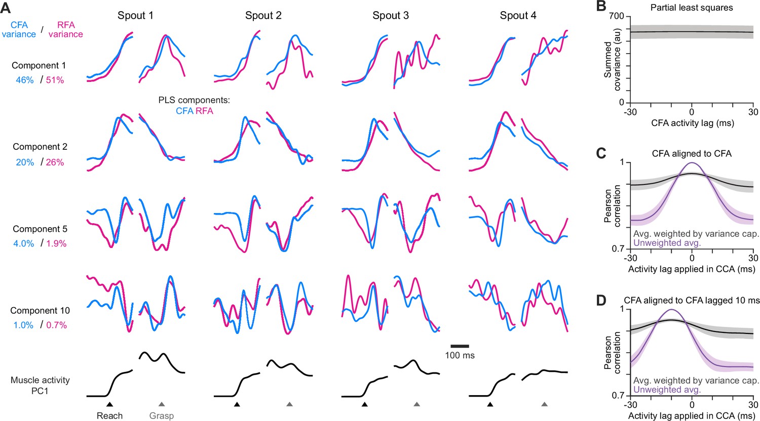
PLS alignment of RFA and CFA activity.
(A) For the same animal used in Figure 4A, four PLS components aligned on reach onset or spout contact (Grasp) for reaches to each spout. Bottom row shows the corresponding time series for the first principal component of muscle activity. (B) Mean ± SEM summed covariance of CFA and RFA PLS components computed when lagging CFA activity relative to RFA. We found no lag where components exhibit an appreciably greater total covariance. (C) Mean ± SEM Pearson correlation of canonical variable pairs computed by aligning CFA activity to itself, but lagging one copy relative to the other, for the average over all pairs either without (purple) or with weighting each correlation value by the variance captured by the given pair (black). (D) Same as (C), but when initially shifting one copy 10ms relative to the other. In this case, we expect the alignment to be maximal at a lag of –10ms.
Figure 5 with 1 supplement
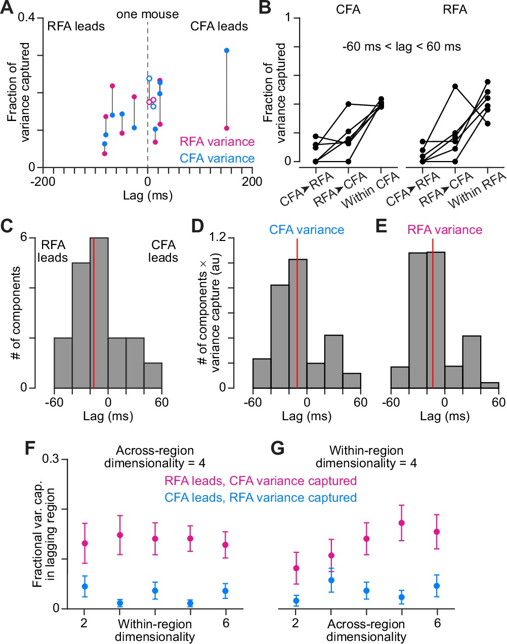
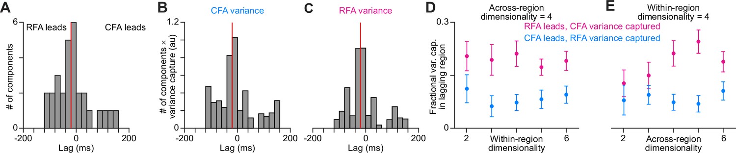
DLAG finds imbalance in variance capture by activity patterns shared at a lag (A).
A scatter plot of the lags of all across-region activity components detected by DLAG versus their fractional variance capture in each region, for one mouse (3 sessions). Open circles reflect components where the lag was not significantly different from zero. Lines connect variance capture for individual components. Values for one component are not shown because its lag failed to converge between –200 and 200ms. (B) Fractional variance capture for CFA activity (left) and RFA activity (right) by across-region components in which CFA activity leads (CFA➤RFA) or RFA activity leads (RFA➤CFA), and by within-region components. Connected dots reflect the average across sessions for individual mice (n=6). (C) Histogram of DLAG component lags that were significantly different from zero and between –60 and 60ms, for all recording sessions (n=15). Red line indicates the median component lag. (D), (E) Histogram of DLAG component lags weighted by the variance each component captures in CFA (D) or RFA (E), for all recording sessions (n=15). Red lines indicate the mean component lag after weighting by variance capture. (F), (G) Mean ± SEM fractional activity variance captured in the lagging region by DLAG components when the lag was significantly different from zero and between –60 and 60ms, when varying the within-region (F) or the across-region (G) dimensionality (n=15 sessions).
Figure 5—figure supplement 1
Additional plots from DLAG calculations.
Results in this figure are similar to Figure 5C–G, but include all components identified by DLAG that have lags between –200 and 200ms. (A) Histogram of DLAG component lags that were significantly different from zero and between –200 and 200ms, for all recording sessions (n=15). Red line indicates the median component lag. (B), (C) Histogram of DLAG component lags weighted by the variance each component captures in CFA (B) or RFA (C), for all recording sessions. Red lines indicate the mean component lag after weighting by variance capture. (D), (E) Mean ± SEM fractional activity variance captured in the lagging region by DLAG components when the lag was significantly different from zero and between –200 and 200ms when varying the within-region (D) or the across-region (E) dimensionality (n=15 sessions).
Figure 6 with 2 supplements

RFA and CFA firing pattern predictivity.
(A,D,G) p-value distributions from calculations of Granger causality (A), transfer entropy (D), and convergent cross mapping (G) using firing patterns of across-region neuron pairs. (B,E,H) For across-region neuron pairs, distributions of metric values reflecting the improved prediction of target neuron firing using source neuron firing (B and E), or the improved prediction of source neuron firing using target neuron firing (H). Here and in (C,F,I), only values for which the corresponding p-value fell below a threshold (set to ensure the false discovery rate = 0.10) are included, and box plots on top show the minimum, 1st, 2nd, and 3rd quartile, and maximum values. (C,F,I) Distributions of metric values computed instead for within-region neuron pairs.
Figure 6—figure supplement 1

Additional plots from firing pattern predictivity calculations.
(A), (B) Firing rate distribution for CFA (blue) and RFA (magenta) neurons belonging to the 10,000 pairs with the highest firing rate product across all 21 recording sessions, before (A) and after (B) applying our algorithm for equalizing the firing rate distributions to avoid imparting a directional bias in firing pattern prediction calculations. Box plots on top show the minimum, 1st, 2nd, and 3rd quartiles, and maximum values.
Figure 6—figure supplement 2

Further neuron pair exclusion to avoid calculation anomalies.
(A) Illustrates the calculation of a firing rate product threshold to eliminate an abnormal number of p values near 1. We determined that these anomalous values resulted from pairs with lower firing rate products, for which statistical assumptions of calculations likely were not met. Trace shows the fraction of p values greater than 0.95 at different firing rate product thresholds on the pairs used for Granger causality calculations. Red line shows the expected fraction greater than 0.95 based on the p value distribution. (B), (C) Firing rate distribution for CFA and RFA neurons included in pairs analyzed using Granger causality (B) or convergent cross mapping (C) after firing rate product threshold exclusion. In (B), (C), box plots on top show the minimum, 1st, 2nd, and 3rd quartiles, and maximum values.
Figure 7

Network modeling of RFA and CFA activity.
(A) Schematic of the dual network model fit to activity measurements. (B) Illustration of fit quality for one instance of the model with unconstrained weights of across-region synapses. In (B) and (E), cyan bars show the epochs of simulated inactivation. (C) Distribution of synaptic weights for all across-region connections from all instances of the unconstrained model. In (C), (D), and (F), box plots show the minimum, 1st, 2nd, and 3rd quartile, and maximum values. (D) Box plots for the distribution of error across 30 instances each of the unconstrained and constrained models. (E) Illustration of fit quality for one instance of the model with across-region weights constrained to be equal in each direction on average. (F) Distributions of summed across-region input (weights x activity) in each direction over different simulation epochs, for all instances of both the unconstrained and symmetric model types. (G) Distributions of within-region excitatory (Excit) and inhibitory (Inhib) synaptic weights, for all instances of both the unconstrained and symmetric model types.
Videos
Video 1
Water reaching, side view.
A side view of a mouse completing a trial of the water reaching task. LEDs are hidden behind the water ports from this view angle.
Video 2
Water reaching, rear view.
A rear view of a mouse completing three trials of the water reaching task. LEDs can be seen in the middle of the screen. Graphics indicate when the LED, Go cue tone (‘Cue’), and water dispensation (‘Reward’) occur. Rewards are achieved when the mouse maintains its hand on the rung for the duration of the rest period.
Additional files
Download links
A two-part list of links to download the article, or parts of the article, in various formats.
Downloads (link to download the article as PDF)
Open citations (links to open the citations from this article in various online reference manager services)
Cite this article (links to download the citations from this article in formats compatible with various reference manager tools)
Hierarchy between forelimb premotor and primary motor cortices and its manifestation in their firing patterns
eLife 13:RP103069.
https://doi.org/10.7554/eLife.103069.3


