Humans adapt rationally to approximate estimates of uncertainty
- Department of Psychiatry, University of Oxford, United Kingdom
- Oxford Health NHS Trust, United Kingdom
Figures
Figure 1
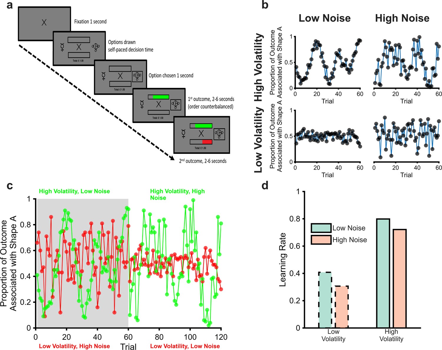
The magnitude learning task (a) Timeline of one trial from the learning task.
On each trial, participants were presented with two abstract shapes and were asked to choose one of them. The empty bars above and below the fixation cross represented the total available wins and losses for the trial, the full length of each bar was equivalent to £1. Participants chose a shape and then were shown the proportion of each outcome that was associated with their chosen shape as coloured regions of the bars (green for wins and red for losses). The empty portions of the bars indicated the win and loss magnitudes associated with the unchosen option, allowing participants to infer which shape would have been the better option on every trial. The task consisted of six blocks of sixty trials each. The volatility and noise of the two outcomes varied independently between blocks with different shapes used in each block. Panel (b) illustrates outcomes from the four block types. As can be seen, blocks with high volatility and low noise (top left), and those with low volatility and high noise (bottom right), present participants with a similar range of magnitudes. Participants, therefore, have to distinguish whether variability in the outcomes is caused by volatility or noise from the temporal structure of the outcomes rather than the size of changes in magnitude (cf. Diederen and Schultz, 2015; Krishnamurthy et al., 2017; Nassar et al., 2012). Panel (c) shows two example blocks (one block in grey, the other in white) with both win (green) and loss outcomes (red) displayed. Panel (d) shows the expected adaptation of learning rates in response to the manipulation of volatility and noise; for both win and loss outcomes, learning rates should be increased when volatility is high and when noise is low.
Figure 2 with 3 supplements
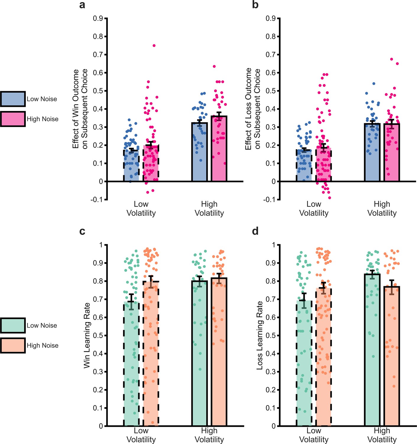
The impact of uncertainty manipulations on participant choice.
Panels a and b report a summary metric for the effect of win and loss outcomes on subsequent choice. The metric was calculated as the proportion of trials in which an outcome of magnitude 51–65 associated with Shape A was followed by choice of the shape prompted by the outcome (i.e. Shape A for win outcomes, Shape B for loss outcomes) relative to when the outcome magnitude was 49–35 (see Methods and materials for more details). We focused on this outcome range as these range of magnitudes were covered by all volatility × noise conditions and it was dictated by the relatively smaller range coverage in the low volatility low noise condition (also see Figure 1C, loss outcomes shown in red between trials 60–120). The higher this number, the greater the tendency for a participant to choose the shape prompted by an outcome. As can be seen, the outcome of previous trials had a greater influence on participant choice when volatility was high, with a small effect of noise, in the opposite direction to that predicted. Panels c and d report the win and loss learning rates estimated from the same data. Again, the expected effect of volatility is observed, this time with no consistent effect of noise. Bars represent the mean (± SEM) of the data, with individual data points superimposed.
Figure 2—figure supplement 1
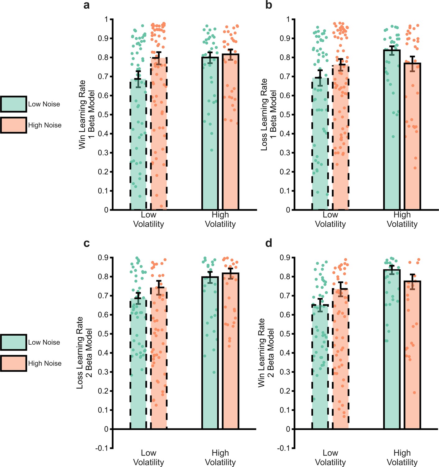
Comparison of estimated win and loss learning rates from the two estimation reinforcement learning (RL) models.
Panels (a) and (b) are the same as panels (c and d) from main Figure 2 and report the estimated win and loss learning rates using the two learning rate one beta model described in the main paper. Panels c and d report the same parameters from the tw0 learning rate two beta model described above. As can be seen, the results are similar regardless of the form of the measurement model used.
Figure 2—figure supplement 2
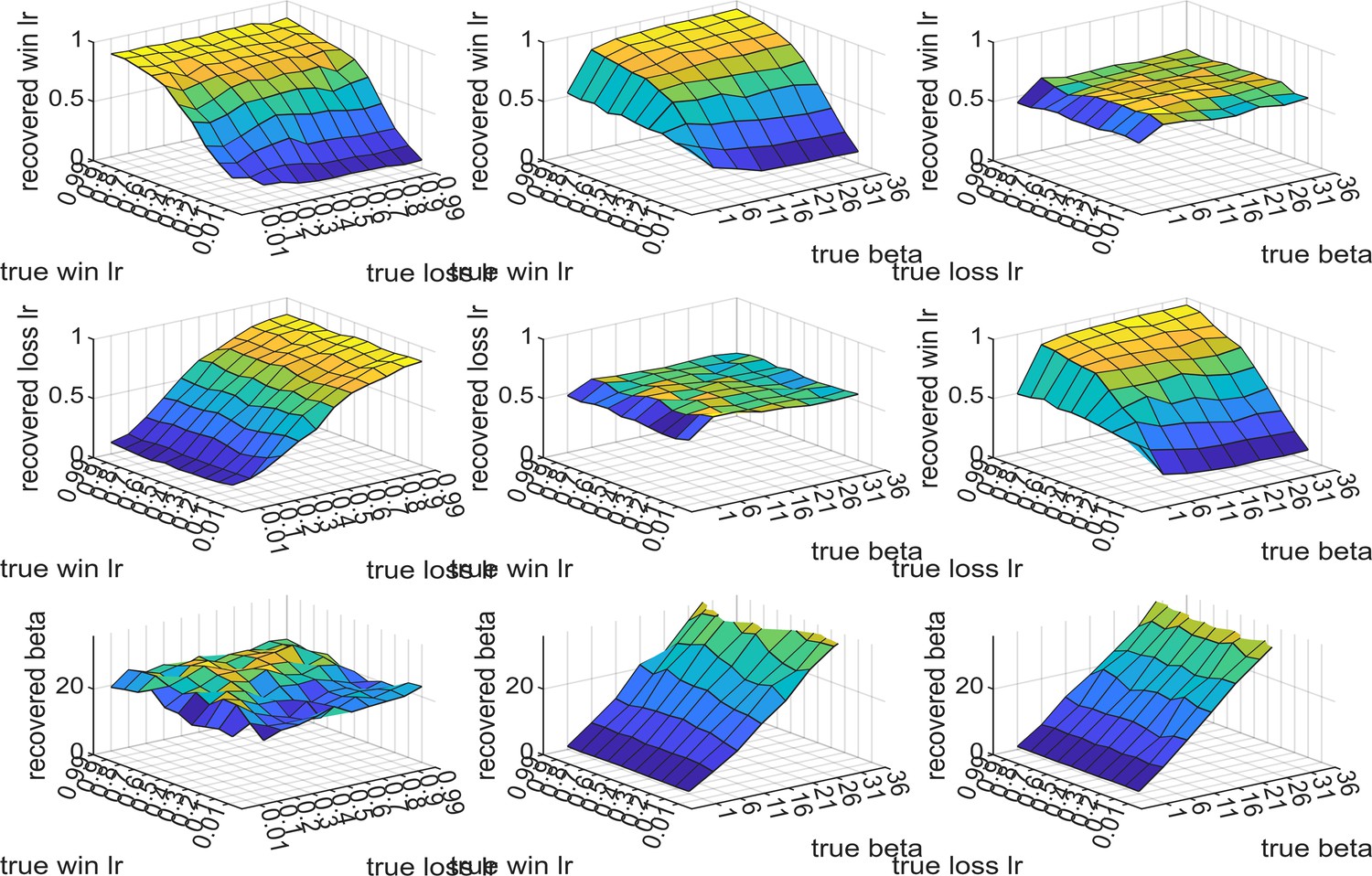
Results of the generate-recover procedure for the reinforcement learning (RL) measurement model.
The two learning rate parameters were varied from 0.01 to 0.99 and the inverse temperature parameter from 1 to 36. Synthetic choices from one task block were generated using the RL model described in the main paper, which were then passed through the model fitting procedure. The recovered parameter values are reported on the z-axis of the plots (the top row reports recovered win learning rates, middle row recovered loss learning rates, bottom row recovered beta values) as a function of different pairs of input parameters (as described on the x and y axes). As can be seen, all three parameters are well recovered, whenever the beta value is above 1.
Figure 2—figure supplement 3
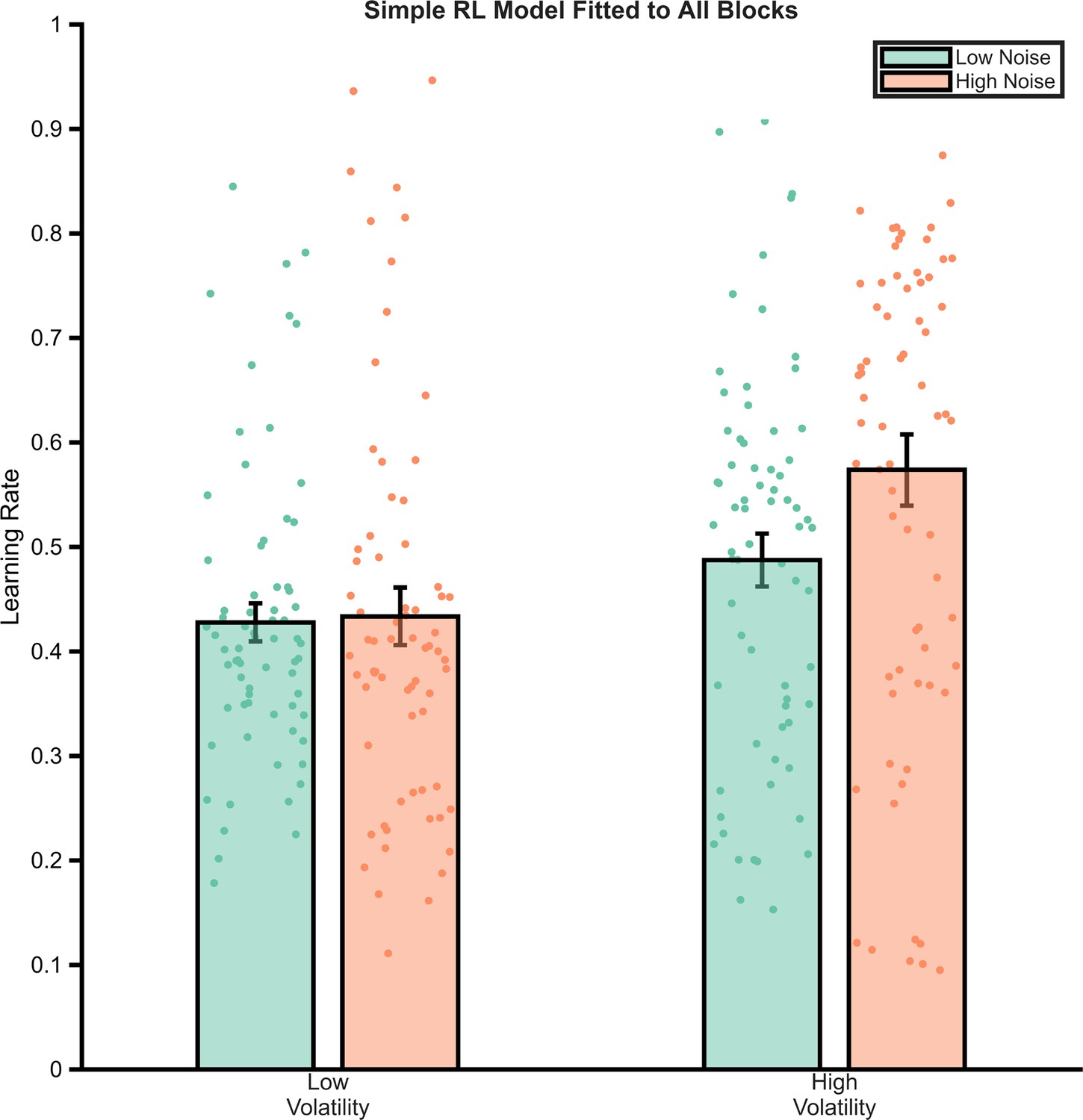
Behaviour of a simple reinforcement learning (RL) model fit across all task blocks.
A three-parameter (win learning rate, loss learning rate, inverse temperature) model was fit to participant’s choices across all blocks. The effective learning rates of the model’s choices are illustrated, demonstrating that it does not replicate the pattern of behaviour seen in participants.
Figure 3 with 1 supplement
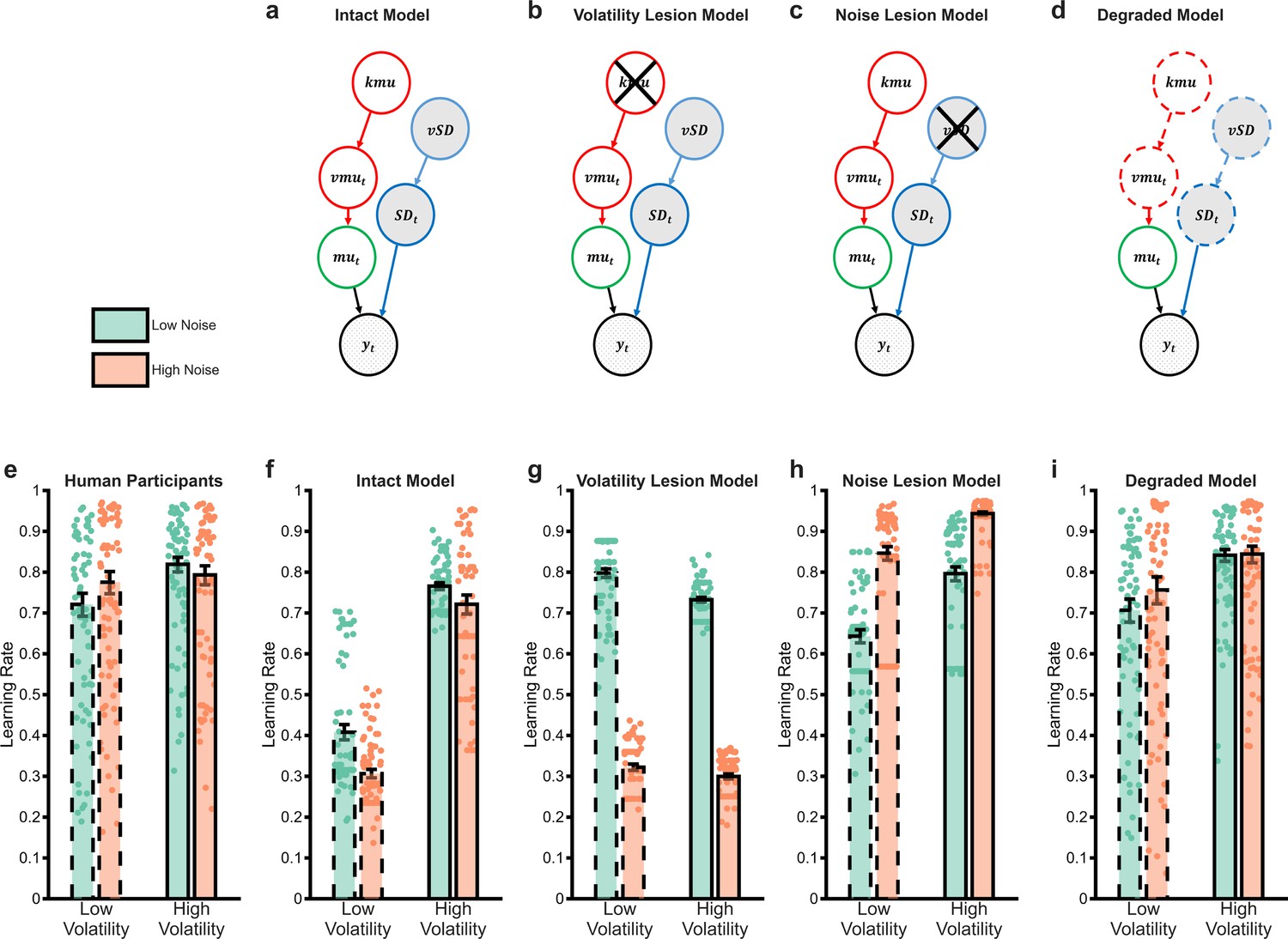
The behaviour of Bayesian observer models.
Bayesian Observer Models (BOM) invert generative descriptions of a process, indicating how an idealised observer may learn. We developed a BOM based on the generative model of the task we used (a) Details of the BOM are provided in the methods, briefly, it assumes that observations () are generated from a Gaussian distribution with a mean () and standard deviation (). Between observations, the mean changes with the rate of change controlled by the volatility parameter (). The standard deviation and volatility of this model estimate the noise and volatility described for the task. The last parameters control the change in volatility () and standard deviation () between observations, allowing the model to account for different periods when these types of uncertainty are high and others when they are low. The BOM adjusts its learning rate in a normative fashion (f), increasing it when volatility is higher, or noise is lower. The BOM was lesioned in a number of different ways in an attempt to recapitulate the learning rate adaptation observed in participants (shown in panel e). Removing the ability of the BOM to adapt to changes in volatility (b) or noise (c) did not achieve this goal (g, h). However, degrading the BOMs representation of uncertainty (d) was able to recapitulate the behavioural pattern of participants (i) Bars represent the mean (± SEM) of participant learning rates, with raw data points presented as circles behind each bar.
Figure 3—figure supplement 1

Analysis of the behaviour of the latent-state model.
The latent-state model described by Cochran and Cisler, 2019 was fit to participant data. Panel a illustrates the behaviour of the fitted model analysed using the reinforcement learning measurement model (main paper Figure 3e–i). As can be seen the model captures the increase in learning rate in high-volatile blocks seen in participants (main paper Figure 3e), but unlike participants increases its learning rate when noise is high. Panel b illustrates the analysis of participant choice data, using model-defined labels of high/low volatility/noise (cf main paper Figure 4d–f). Where the degraded Bayesian observer model (BOM) rescued the normative behaviour of participants (main paper Figure 4f), the latent-state model does not.
Figure 4 with 2 supplements
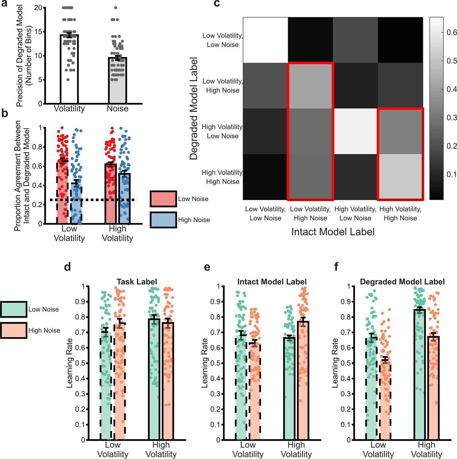
Analysis of the behaviour of the degraded Bayesian observer model (BOM).
The process of degrading the BOM involved reducing the number of bins used to represent the volatility and noise dimensions independently until the choice of the model matched that of participants. Panel (a) illustrates the number of bins selected by this process for the volatility and noise dimensions (averaged across win and loss outcomes). As can be seen, the degraded BOM maintained a less precise representation of noise than volatility. In order to understand the behaviour of the degraded model, the model’s estimated and were used to label individual trials as high/low volatility and noise (NB greater than or less than the mean value of the estimates). These trial labels were compared with the same labels from the intact model, which were used as an ideal comparator (panels b and c). Panel b illustrates the proportion of trials in which the labels of the two models agreed, arranged by the ground truth labels of the full model and averaged across win and loss outcomes. The dotted line indicates the agreement expected by chance. The degraded model trial labels differed from those of the full model particularly for high noise trials, with no impact of trial volatility. Panel c provides more details on how the degraded model misattributes trials. In this figure, the labels assigned by the full model are arranged along the x-axis. The colour of each square represents the proportion of trials with a specific full model label that received the indicated label of the degraded model (arranged along the y-axis). The diagonal squares illustrate agreement between models as reported in panel (b). As highlighted by the red outlines, trials which the full model labelled as having high noise were generally mislabelled by the degraded model as having high volatility. Reanalysis of participant choices using the trial labels provided by the full (panel e) and degraded (panel f) models indicates that participants adapt their learning rates in a normative fashion when the degraded model trial labels are used (panel f), but not when the full model labels are used (panel e). Panel (d) illustrates the same analysis using the original task block labels for comparison. Bars represent the mean (± SEM) of participant learning rates, with raw data points presented as circles behind each bar. See Figure 4—figure supplement 1 for a comparison of the behaviour of the degraded BOM with an alternative fitted model.
Figure 4—figure supplement 1
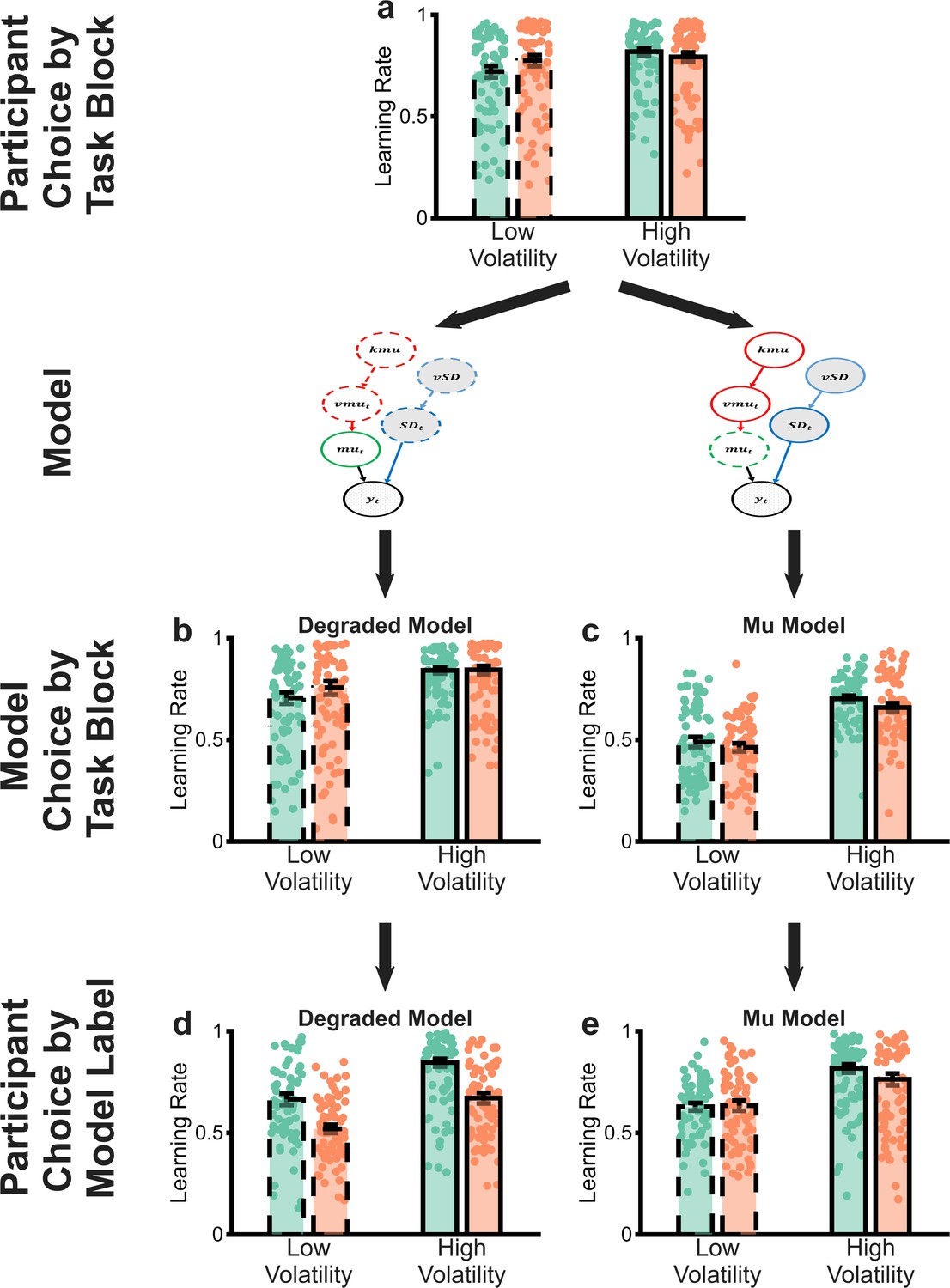
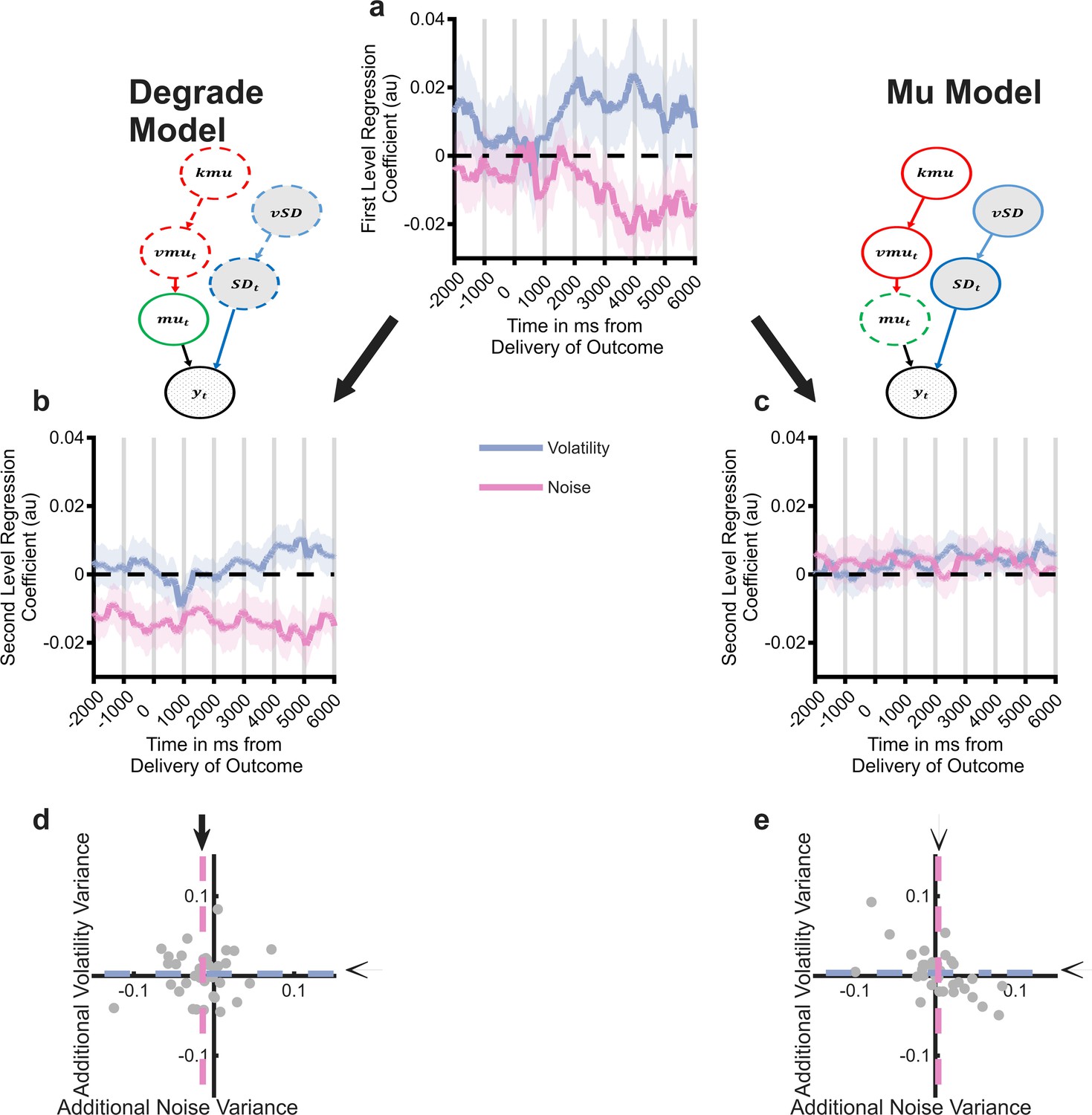
Comparison of the degraded volatility/noise Bayesian observer model (BOM) and a control model (‘mu model’) in which the representation of the mean of the generative process, rather than the volatility/noise are degraded.
Panel a illustrates the behaviour of participants in the task (as reported in main text Figure 2). Panel b illustrates the behaviour of the degraded volatility/noise model (as reported in main text Figure 3) and panel d illustrates that participants are behaving normatively if we assume that they are using a similar estimate of volatility and noise as the degraded volatility/noise model (as reported in main text Figure 4). Panel c illustrates that the mu model does not recapitulate participant behaviour and panel e shows that, assuming participants use similar estimates of volatility/noise as the mu model does not rescue normative behaviour.
Figure 4—figure supplement 2
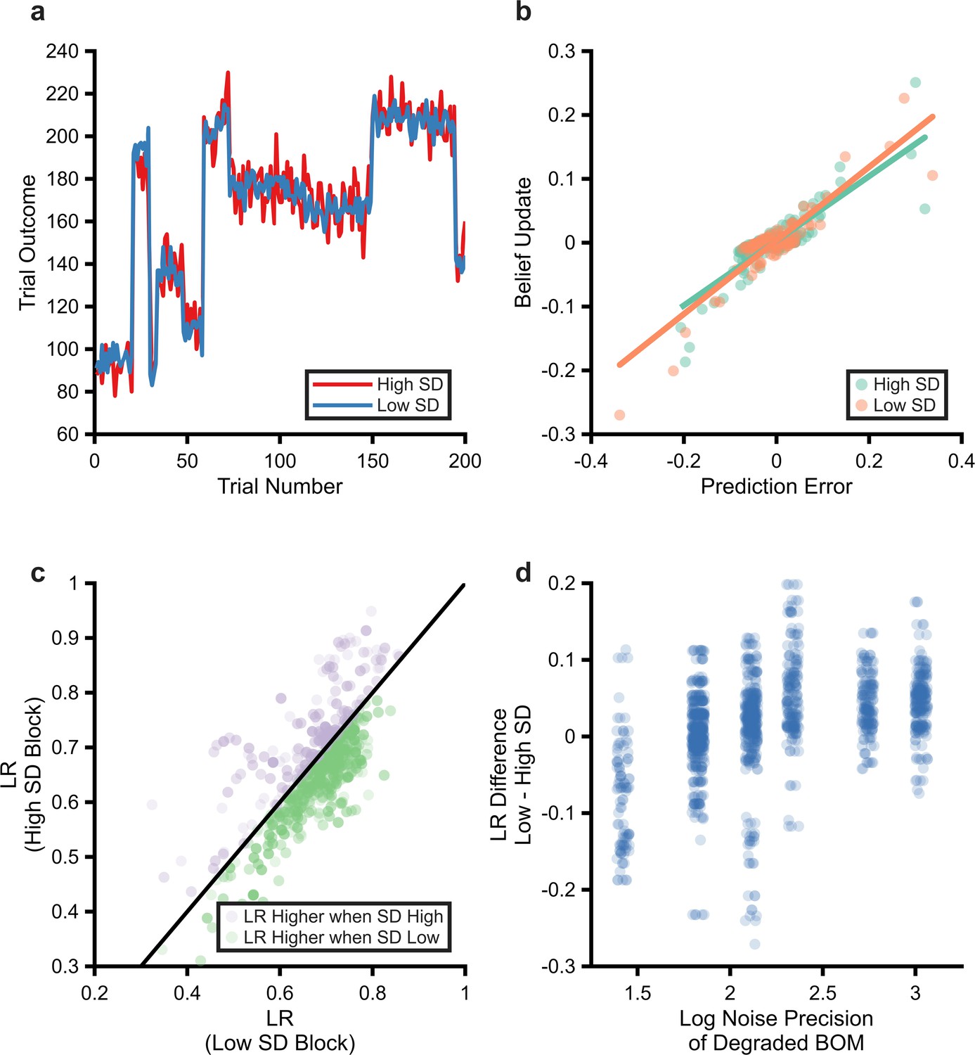
Performance of the degraded Bayesian observer model (BOM) on schedules derived from Nassar et al., 2012.
Example high and low noise schedules used (panel a, blue line low noise schedule, red line high noise schedule). Volatility is generated by jumps in the mean of the generative process that occur with a probability of 0.1 on each trial, after at least three trials have passed since the last jump. Noise is added by drawing samples from a Gaussian distribution centred on this mean, using an SD of either 10 (high SD) or 5 (low SD). As can be seen, changes in the magnitude of the outcome produced by volatility are substantially larger than those caused by noise. The performance of the degraded BOM on this task was estimated by passing generated schedules from this task to the BOM (using the noise/volatility bins estimated for participants in the current study, 20 schedules were used per participant). Estimating learning rate from the task for a specific individual and schedule (panel b). Unlike the task reported in the current paper, the outcome of the Nassar et al. paper was continuous (the subsequent value was predicted). This allows the effective learning rate used in high and low SD blocks to be estimated as the slope of the line linking trialwise belief update (i.e. change in prediction of the model) and prediction error. The degraded model uses a higher learning rate when noise is low than when it is high in the Nassar task (panel c). The estimated learning rates for high and low SD blocks illustrated for all participants and all schedules. As can be seen, and as reported by Nassar et al., the degraded model uses a higher learning rate when SD is small (t(69)=3.6, p=0.0006). The degree to which the degraded BOM increased its learning rate in low relative to high SD blocks was significantly associated with the precision with which it represented noise (panel d).
Figure 5 with 1 supplement
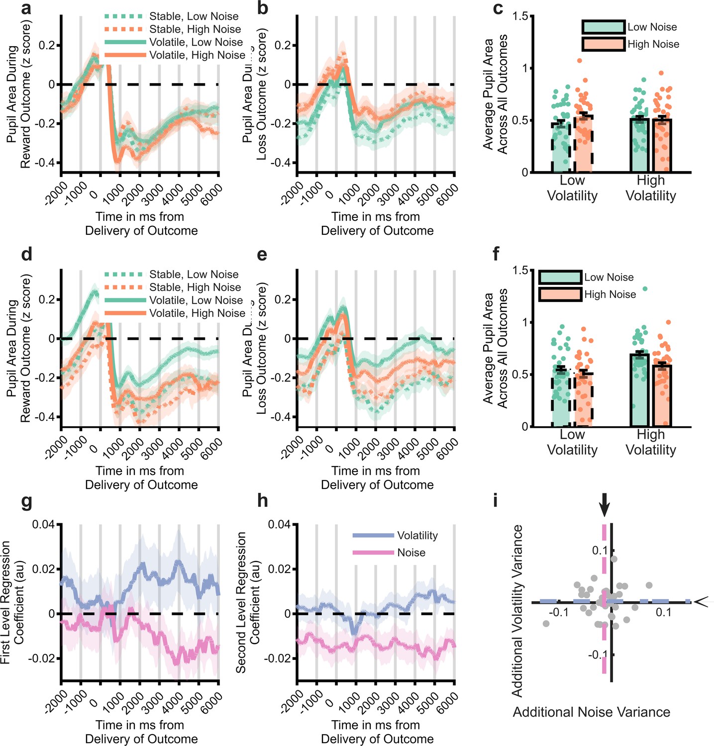
Analysis of pupillometry data.
Z-scored pupil area from 2 s before to 6 s after win (panel a) and loss (panel b) outcomes, split by task block. Lines illustrate average size, with shaded area illustrating SEM. Panel c Pupil size averaged across whole outcome period and both win and loss outcomes. Pupil size did not systematically vary by task block. Panels (d-f) as above but using the trial labels derived from the degraded model. Pupil size was significantly larger for trials labelled as having high vs. low volatility and low vs. high noise. Panel (g) displays the mean (SEM) effect of volatility and noise as estimated by the full BOM derived from a regression analysis of pupil data. The residuals from this analysis were then regressed against the estimated volatility and noise from the degraded model. A time course of the regression weights from this analysis is shown in panel h, with the mean coefficients across the whole period shown in panel i. The degraded model’s estimated noise accounted for a significant amount of variance not captured by the full model (pink line in h is below 0, the mean effect across the period is represented by dashed lines and arrows in panel i). See Figure 5—figure supplement 1 for comparison of the degraded BOM with an alternative fitted model.
Figure 5—figure supplement 1
Comparison of the degraded volatility/noise Bayesian observer model (BOM) and the mu BOM on analysis of the pupillometry data.
As reported in main Figure 5, the intact BOM explains variance in pupil signal attributable to both volatility and noise (panel a), with the degraded BOM explaining additional variance over and above this, attributable to noise (panels b and d). In contrast, the mu model does not explain additional variance over and above the full model (panels c and e).
Videos
Animation 1
Estimation of the causes of uncertainty by the Bayesian Observer Model.
Lower right panel: Synthetic data with periods of high (trial number: 0-60; 120-180; 240-360) and low (trial number: 60-120; 180-240) volatility and high (trial number: 180-240) and low (trial number: 1-180; 240-360) noise was provided to the Bayesian Observer Models. The models trial-by-trial estimate of volatility and noise is illustrated by marginalising over all but the vmu and SD dimensions of the joint probability distribution (see description of the Bayesian Observer Model in the methods). This produces a two-dimensional probability density of the model’s estimate of volatility (y-axes) and noise (x-axes). The current data being fed to the model is illustrated by the solid line moving through the data. Top left panel: The estimated uncertainty of the full (unlesioned) model. The model adapts to different periods of high and low volatility reasonably well (e.g. see the period around trial 180 when the data moves from high volatility/low noise to high noise/low volatility). The fully lesioned models are provided for comparison (see methods section for a description of these models). Top right panel: The noise blind model (vSD has been removed) cannot account for changes in noise and so any change in either volatility or noise is captured as a change in volatility. Lower left panel: The volatility blind model (kmu has been removed) cannot account for changes in volatility and so any change in either volatility or noise is captured as a change in noise.
Tables
Table 1
Demographic details of participants.
| Measure | Mean (SD) |
|---|---|
| Age | 29.07 (10.86) |
| Gender | 69% Female |
| QIDS-16 | 5.26 (4.25) |
| Trait-STAI | 36.21 (10.42) |
| State-STAI | 30.29 (8.57) |
-
QIDS-16; Quick Inventory of Depressive Symptoms, 16-item self-report version. Trait/State-STAI; Spielberger State-Trait Anxiety Inventory.
Table 2
Summary of free parameters in latent state model (see Cochran and Cisler, 2019 for detailed description).
| Parameter | Description | Separate for win and loss outcomes | Number of parameters |
|---|---|---|---|
| Alpha0 | Learning rate for the association | yes | 2 |
| Alpha1 | Learning rate for variance | yes | 2 |
| Alpha2 | Learning rate for covariance | yes | 2 |
| Gamma | Transition probability between states | yes | 2 |
| Eta | Threshold for creating new state | yes | 2 |
| Beta | Inverse choice temperature | No | 1 |
Additional files
Download links
A two-part list of links to download the article, or parts of the article, in various formats.
Downloads (link to download the article as PDF)
Open citations (links to open the citations from this article in various online reference manager services)
Cite this article (links to download the citations from this article in formats compatible with various reference manager tools)
Humans adapt rationally to approximate estimates of uncertainty
eLife 14:RP103734.
https://doi.org/10.7554/eLife.103734.3


