Figures and data in Hunger shifts attention and attribute weighting in dietary choice

Figures
Tables
Additional files

38 figures, 13 tables and 2 additional files

Figures

Figure 1

Download asset Open asset

Experimental design.

(a) Food rating task. Participants rated all food images and their corresponding Nutri-Scores (see *Methods*) in terms of taste, health, wanting, and perceived caloric content on a continuous scale (b) Trial sequence of food choice task. In each trial, participants made a binary choice between two food options represented by food image and corresponding Nutri-Scores; Feedback and fixation-based fixation dots were implemented (c) Experimental procedures; blue refers to sated, yellow to hungry condition (order counterbalanced). VAS refers to visual analog scale used to assess subjective feelings of hunger. Positive and negative affect scale (PANAS) refers to a questionnaire assessing mood (see *Appendix 1*). FEV II refers to a questionnaire assessing eating behavior (see *Appendix 2*); *indicates that these steps were only required in the first session.

Figure 2 with 4 supplements

Download asset Open asset

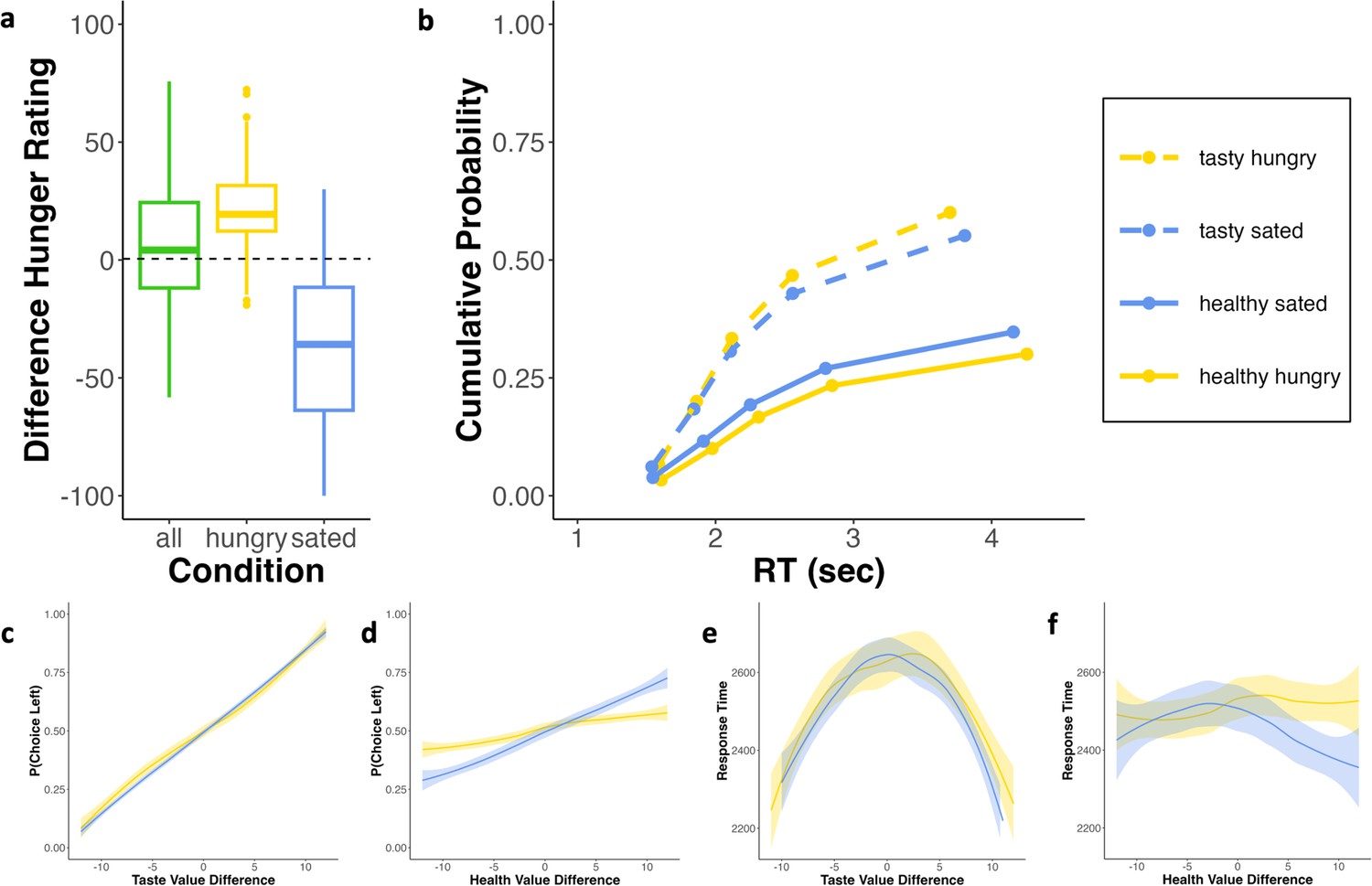
Behavioral results.

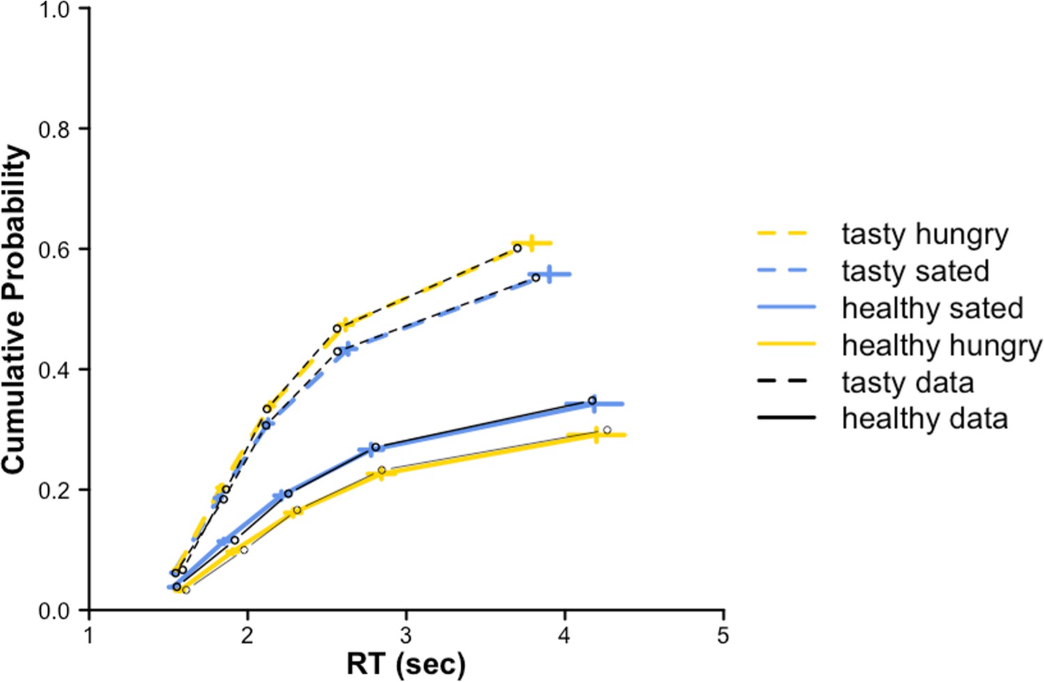
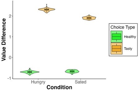
(a) Manipulation check: The green boxplot displays the difference (hungry-sated) in hunger state at arrival at the lab, yellow and blue boxplots display the difference (last timepoint-first timepoint) in hunger state in the hungry and sated condition, respectively. (b) Response time (RT) quantile plot displaying the cumulative probability of tasty (dashed lines) and healthy choices (solid lines) separately for the two conditions (quantiles are 0.1, 0.3, 0.5, 0.7, 0.9 of choices). (**c, d**) Probability to choose the left option as a function of taste and health value difference (left-right), respectively. Importantly, the dependency of choice on health information was eliminated under hunger. (**e, f**) Corresponding mean RTs as a function of taste and health value difference, respectively. For illustration purposes, value differences were segmented into 25 bins, and a locally weighted scatterplot smoothing technique was applied with a span of 0.75. Plots (**c–f**) are based on all trials. Transparent shades indicate the standard errors of the smoothed choice probability and RT for the respective value bins (see also Figure 2—figure supplement 3).

Figure 2—figure supplement 1

Download asset Open asset

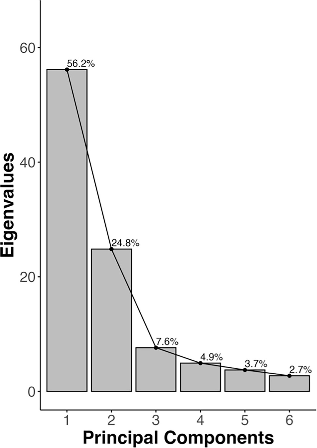
Principal component analysis.

Screeplot, the first component positively loads on health rating and Nutri-Score and negatively on objective and subjective caloric content, the second component positively loads on taste and wanting ratings.

Figure 2—figure supplement 2

Download asset Open asset

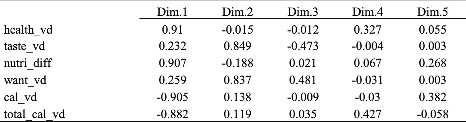
Factor loadings on the components for the respective datasets.

vd refers to value difference left – right option.

Figure 2—figure supplement 2—source data 1 Source table.: https://cdn.elifesciences.org/articles/103736/elife-103736-fig2-figsupp2-data1-v1.docx
Download elife-103736-fig2-figsupp2-data1-v1.docx

Figure 2—figure supplement 3

Download asset Open asset

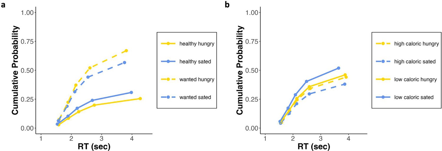
Quantile plots based on wanting and caloric information.

Response time (RT) quantile plot displaying the cumulative probability separately for the two conditions (blue = sated condition and yellow = hungry condition) of (a) higher wanted (dashed lines) and healthy choices (solid lines); and (b) higher caloric (dashed lines) and lower caloric choices (solid lines) (quantiles are 0.1, 0.3, 0.5, 0.7, 0.9 of choices).

Figure 2—figure supplement 4

Download asset Open asset

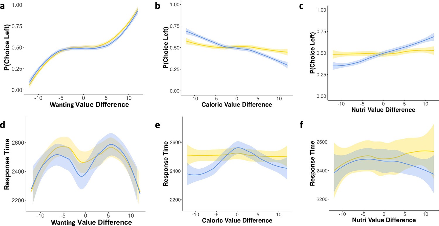
Choice as a function of value difference.

(**a–c**) Probability to choose the left option as a function of wanting, subjective caloric content, and Nutri-Score value difference (left-right), respectively. Higher wanted options increased probability of choice, irrespective of condition. While lower calories and a better Nutri-Score promoted choice in the sated condition, this dependency was eliminated under hunger (**d-f**). Corresponding mean response times (RTs) as a function of wanting, subjective caloric content, and Nutri-Score value difference (left-right), respectively. Importantly, the pattern of the wanting plots (a) and (d) closely corresponds to those of the taste plots (Figure 2c and e), while the pattern of the Nutri-Score plots closely corresponds to those of the health plots (Figure 2d and f). For illustration purposes, value differences were segmented into 25 bins, and a locally weighted scatterplot smoothing technique was applied with a span of 0.75. Plots are based on all trials. Transparent shades indicate the standard errors of the smoothed choice probability and RT for the respective value bins.

Figure 3 with 3 supplements

Download asset Open asset

Eye-tracking results.

(a) Dwell time difference between the tasty and healthy option was positively associated with the probability of choosing the tasty option in both conditions. (b) The average probability to look at food image (taste attribute) compared to Nutri-Score (health attribute) was even higher in the hungry than sated condition. (c) Path diagram with posterior means of the parameters, associated 95%-credible interval in squared brackets.

Figure 3—figure supplement 1

Download asset Open asset

Proportion of first and last fixations.

(a) Proportion (y-axis) of last fixation by category (x-axis) (b) Proportion (y-axis) of first fixation by category (x-axis) (c) Proportion (y-axis) of first fixation by location on the screen (y-axis) (d) Fixation transitions across participants and conditions. In line with the strong tendency to fixate food images, rather than the Nutri-score, participants’ fixations mostly switched within attributes ( $M_{s a t e d} = 0.868$ , $S D_{s a t e d} = 0.14$ ; $M_{h u n g r y} = 0.899$ , $S D_{h u n g r y} = 0.108$ ), with only few transitions within alternatives ( $M_{s a t e d} = 0.096$ , $S D_{s a t e d} = 0.105$ ; $M_{h u n g r y} = 0.073$ , $S D_{h u n g r y} = 0.081$ ), and even fewer transitions being diagonal ( $M_{s a t e d} = 0.037$ , $S D_{s a t e d} = 0.038$ ; $M_{h u n g r y} = 0.028$ , $S D_{h u n g r y} = 0.029$ ). We performed the Wilcoxon rank sum test due to violations against normality, which revealed no differences between conditions across transition types (diagonal: W=2152.5, p=0.216; within alternative: W=2189.5, p=0.279; within attribute: W=2750.5, p=0.211). We further used the Payne index (Payne, 1976) to describe participants’ search patterns, confirming that search was mostly attribute-based: hungry participants had a Payne index of –0.846 ( $S D_{h u n g r y} = 0.178$ ) and sated participants one of –0.793 ( $S D_{s a t e d} = 0.234$ ), with no difference between conditions (W=2189.5, p=0.279). Blue indicates sated condition, yellow indicates hungry condition.

Figure 3—figure supplement 2

Download asset Open asset

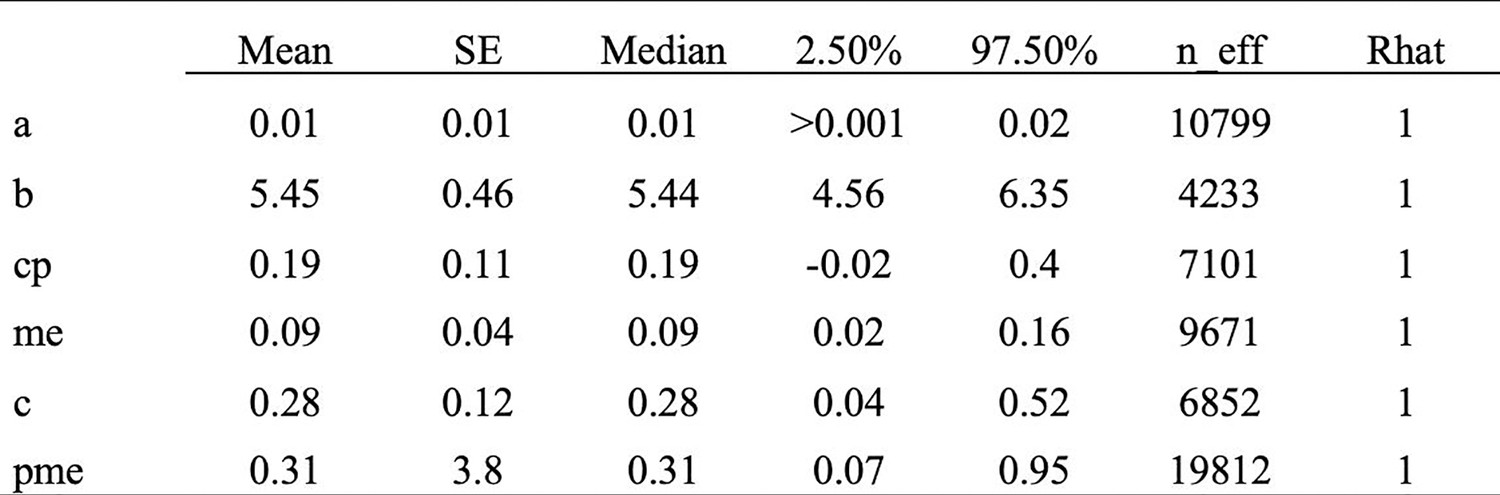
Mediation coefficients.

a is the effect of hunger state to attention, b is the effect from attention to choice, cp is the indirect effect of hunger state on choice taking attention into account, c is the direct effect of hunger state on choice, when not considering attention, me refers to the mediation effect, thus the combination of paths a and b, *pme* refers to the proportion of the effect that is mediated. Output refers to posterior, mean, standard deviation (=standard error; SE), median, and credible interval respectively. n_eff refers to the number of effective posterior samples, to obtain confident estimates, it is recommended to be >100 Vuorre and Bolger, 2018; R-hat is the scale reduction factor, to accurately predict posterior distributions, it should be 1.00, according to Vuorre and Bolger, 2018 values within 0.05 are acceptable.

Figure 3—figure supplement 2—source data 1 Source table.: https://cdn.elifesciences.org/articles/103736/elife-103736-fig3-figsupp2-data1-v1.docx
Download elife-103736-fig3-figsupp2-data1-v1.docx

Figure 3—figure supplement 3

Download asset Open asset

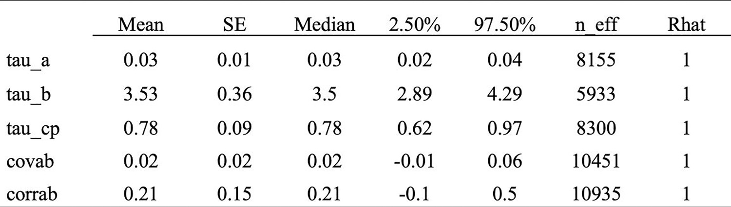
Standard deviations of subject-level effects (random effects), their covariances, and correlations.

Figure 3—figure supplement 3—source data 1 Source table.: https://cdn.elifesciences.org/articles/103736/elife-103736-fig3-figsupp3-data1-v1.docx
Download elife-103736-fig3-figsupp3-data1-v1.docx

Figure 4 with 1 supplement

Download asset Open asset

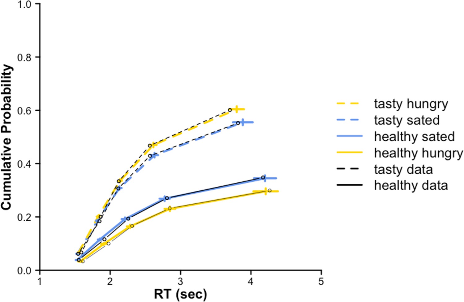
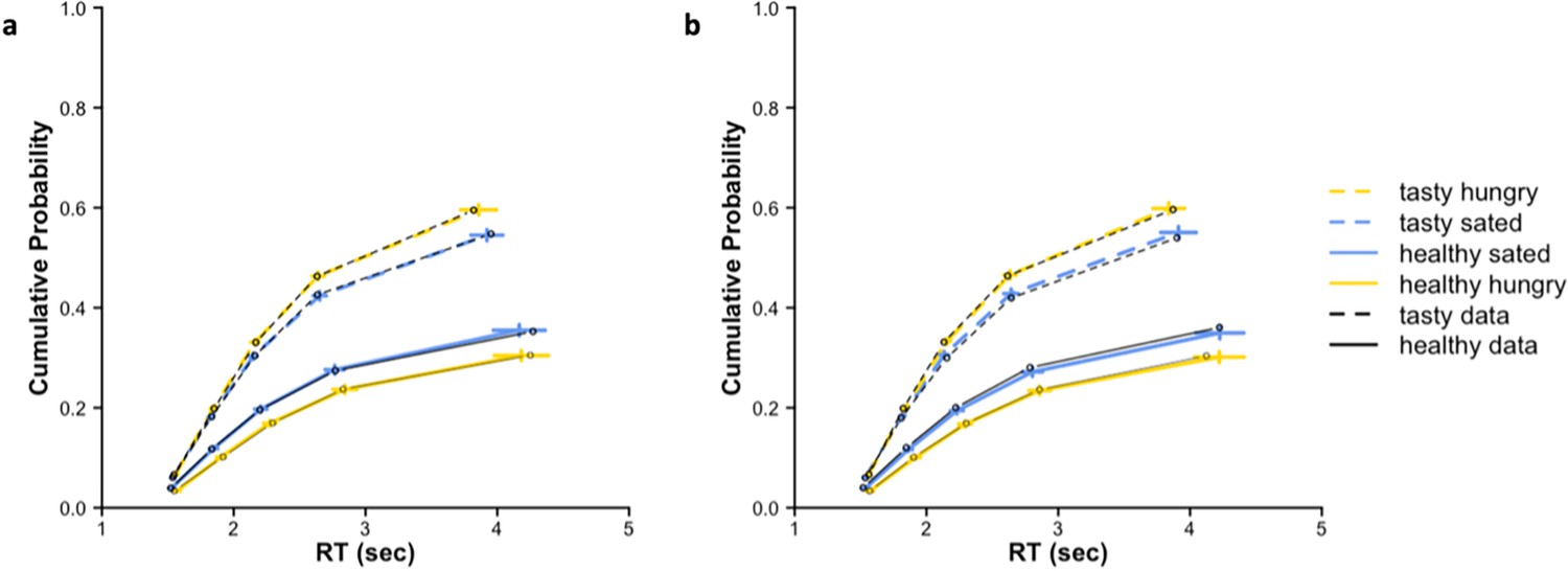
Posterior predictive checks maaDDM2 $ϕ$ .

Quantile plots of simulated data with fitted parameters of the maaDDM2 $ϕ$ in blue (sated) and yellow (hungry) with highest density intervals (HDI) of each quantile (vertical lines) and behavior. Posterior predictive checks were performed by drawing 1000 parameter values from the individual posterior parameter distribution to simulate the new data.

Figure 4—figure supplement 1

Download asset Open asset

Posterior predictive checks for multi-attribute attentional DDM (maaDDM).

Quantile plots of simulated data with fitted parameters of the maaDDM in blue (sated) and yellow (hungry) with highest density intervals (HDI) of each quantile (vertical lines) and behavior. Posterior predictive checks were performed by drawing 1000 parameter values from the individual posterior parameter distribution to simulate the new data.

Figure 5 with 1 supplement

Download asset Open asset

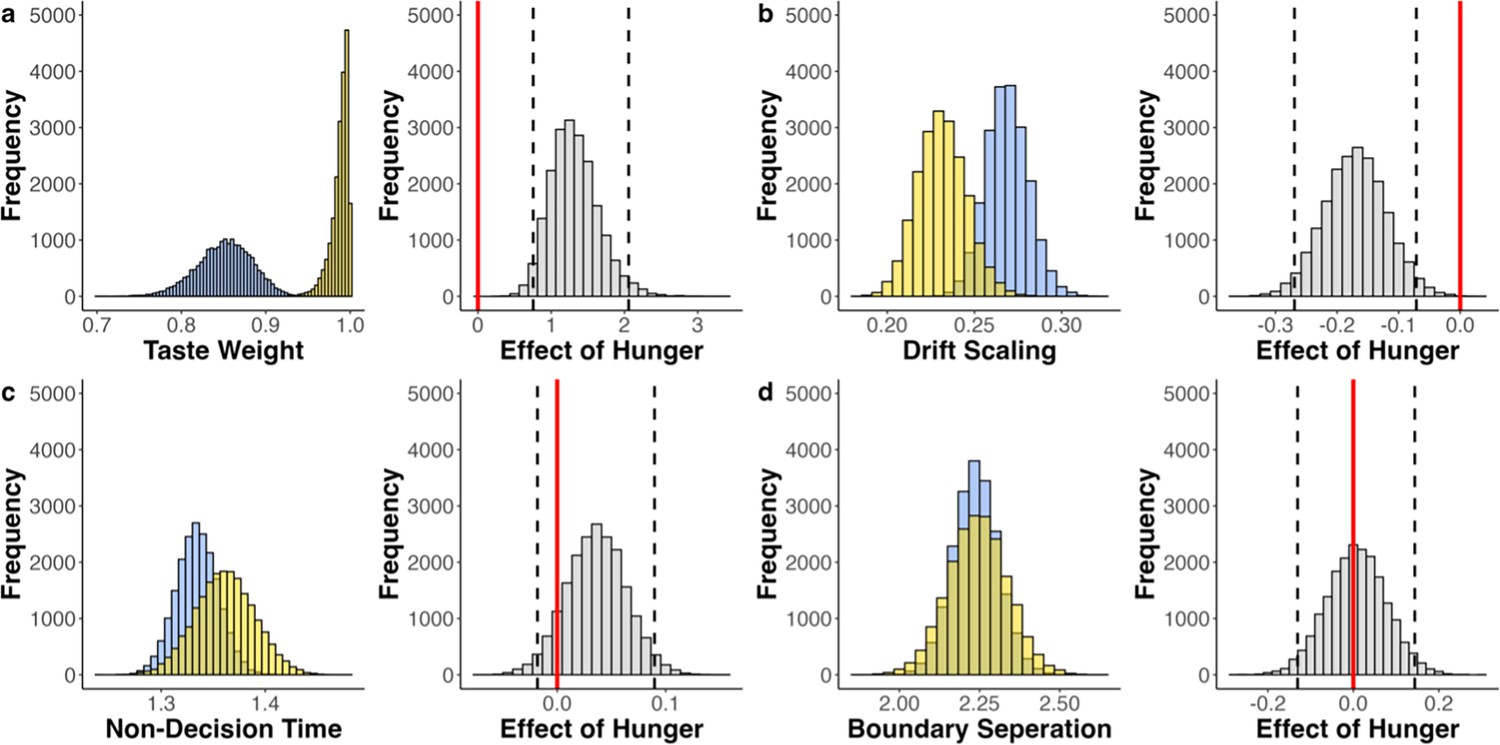
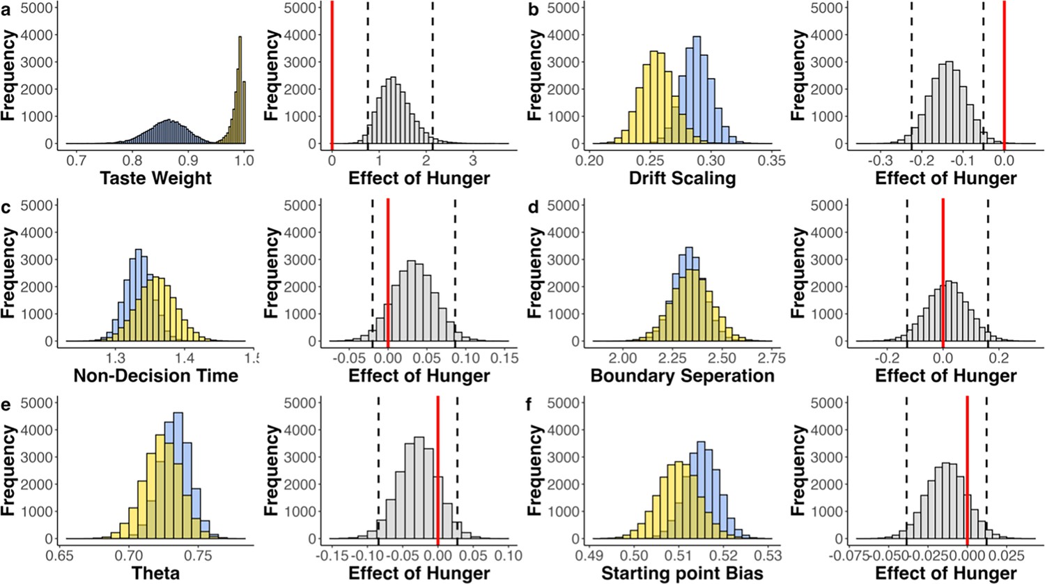
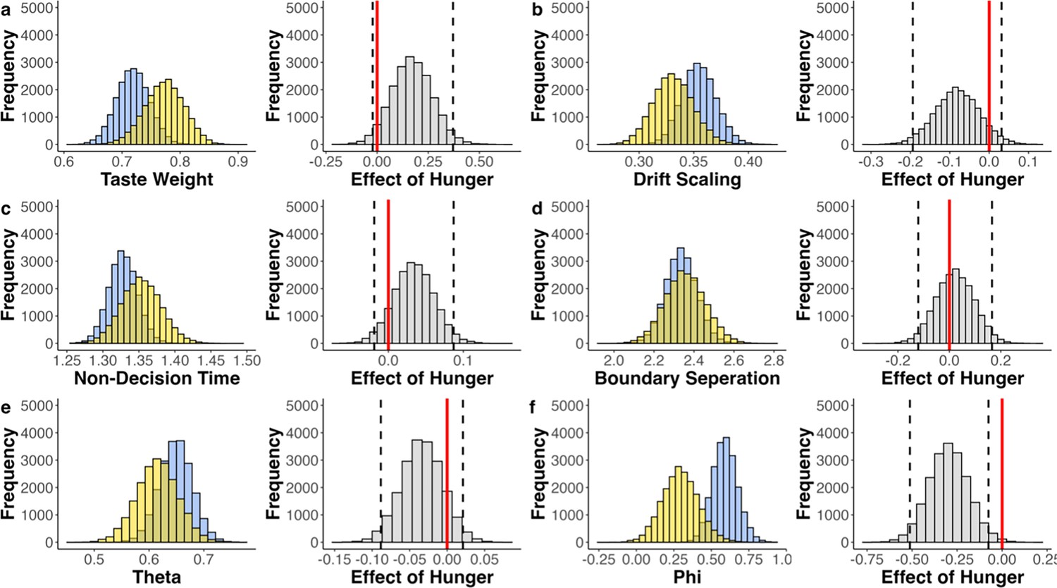
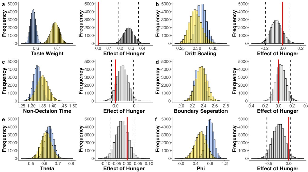
Parameter estimates of maaDDM2 $ϕ$ .

Group parameter estimates (blue = sated, yellow = hungry; left panels) and the effect of hunger state (gray; right panels). Dashed black lines indicate the 95% HDI. (a) Estimated taste weights. In both conditions the weight is larger than 0.5, indicating a higher weight on taste compared to health. This preference was even stronger under hunger. (**b–f**) Parameter estimates of $d$ , nDT, $α$ , $θ$ and $ϕ_{T}$ , and the corresponding effects of hunger state. (g) Parameter estimates of $ϕ_{H}$ and the corresponding effects of hunger state, showing that the attention-driven discounting of health information was amplified under hunger.

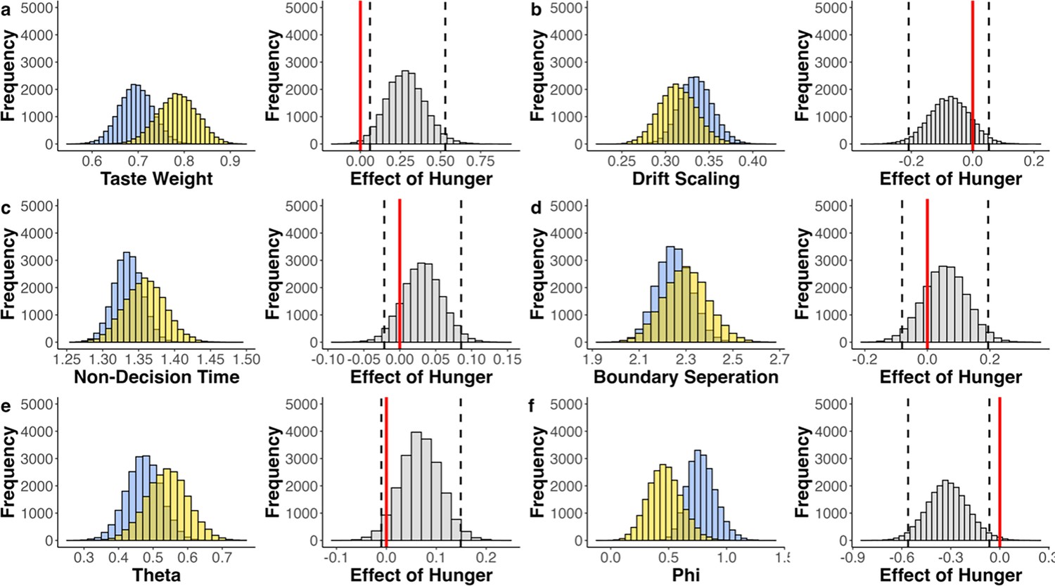
Figure 5—figure supplement 1

Download asset Open asset

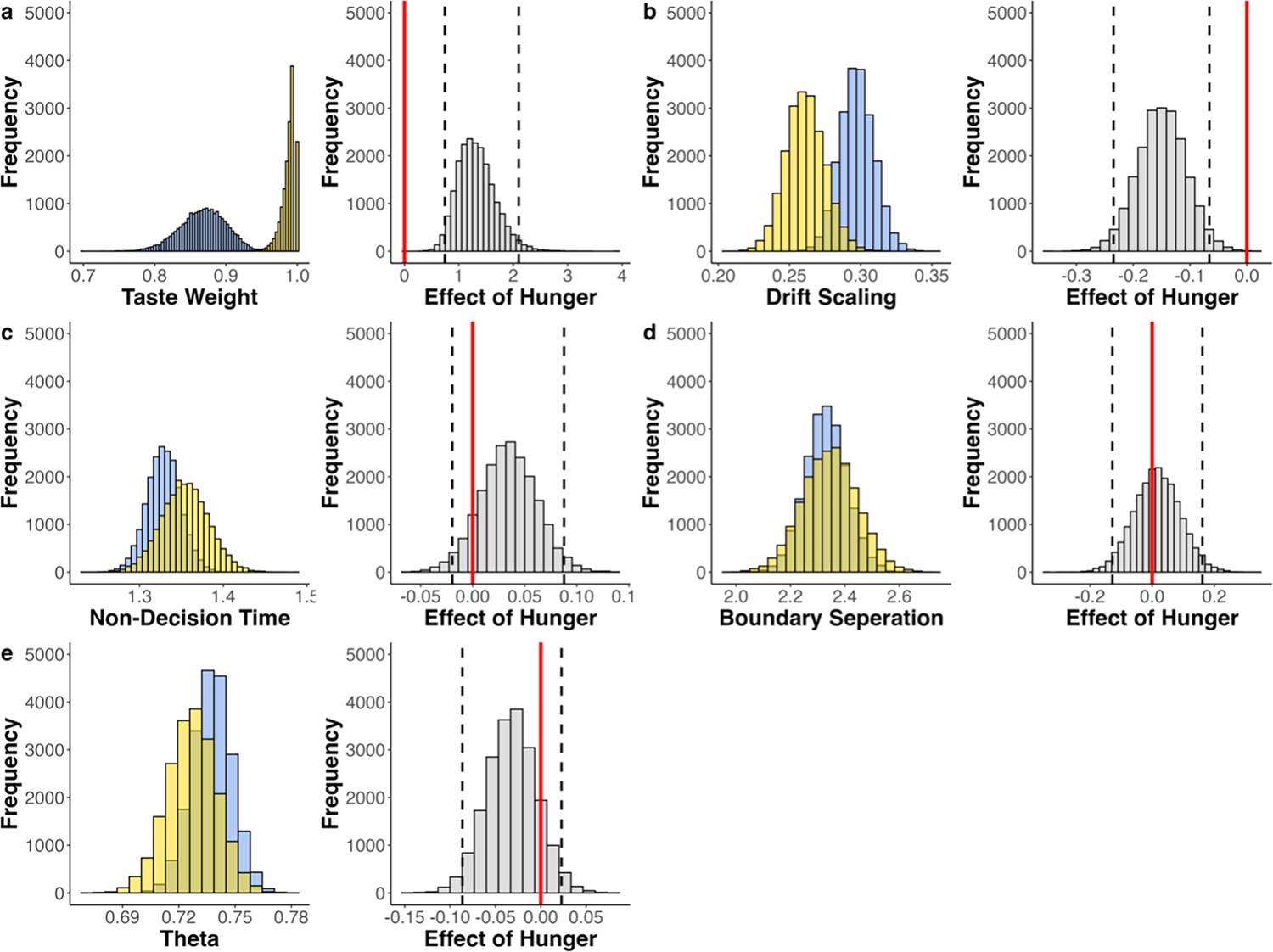
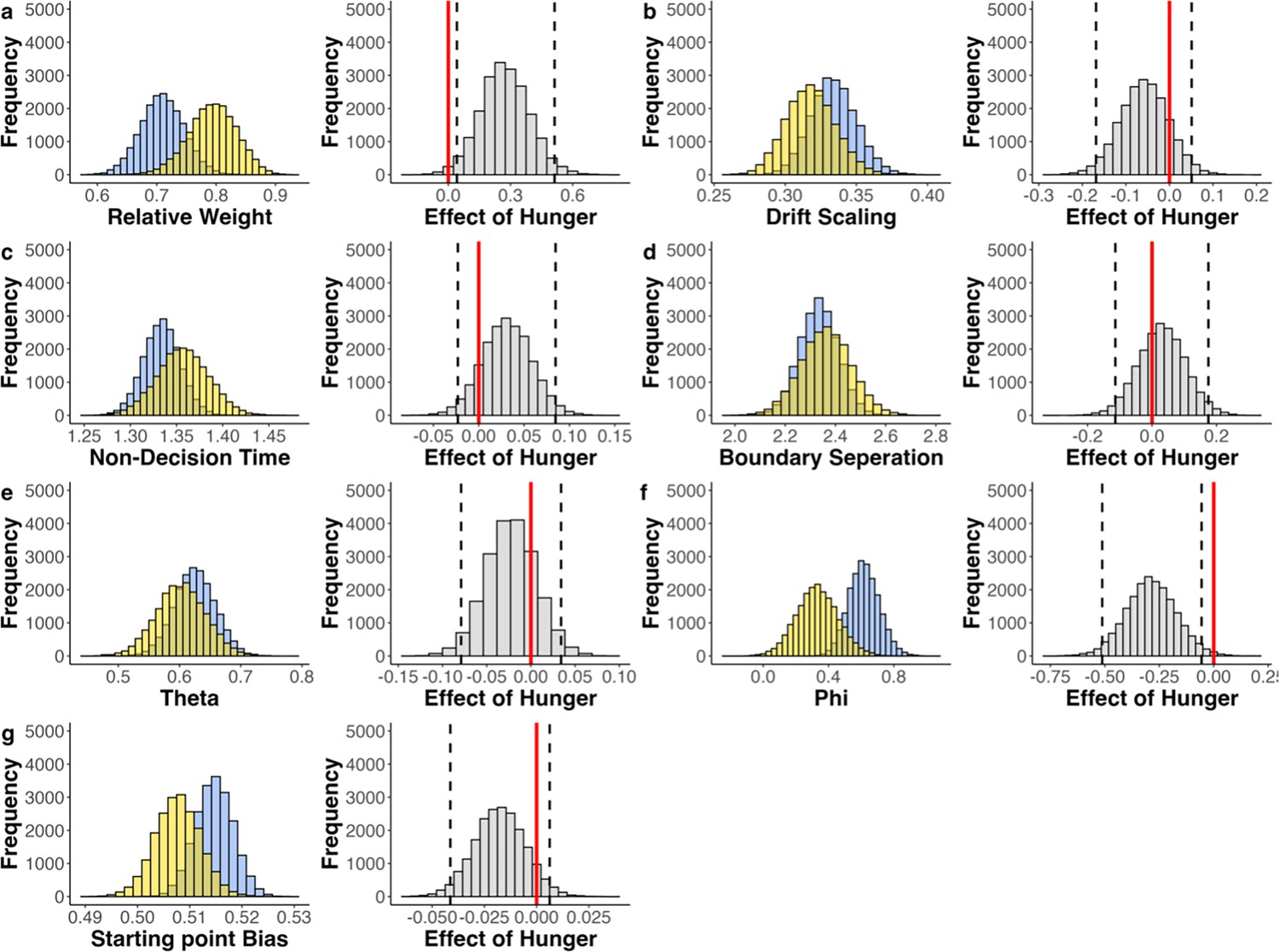
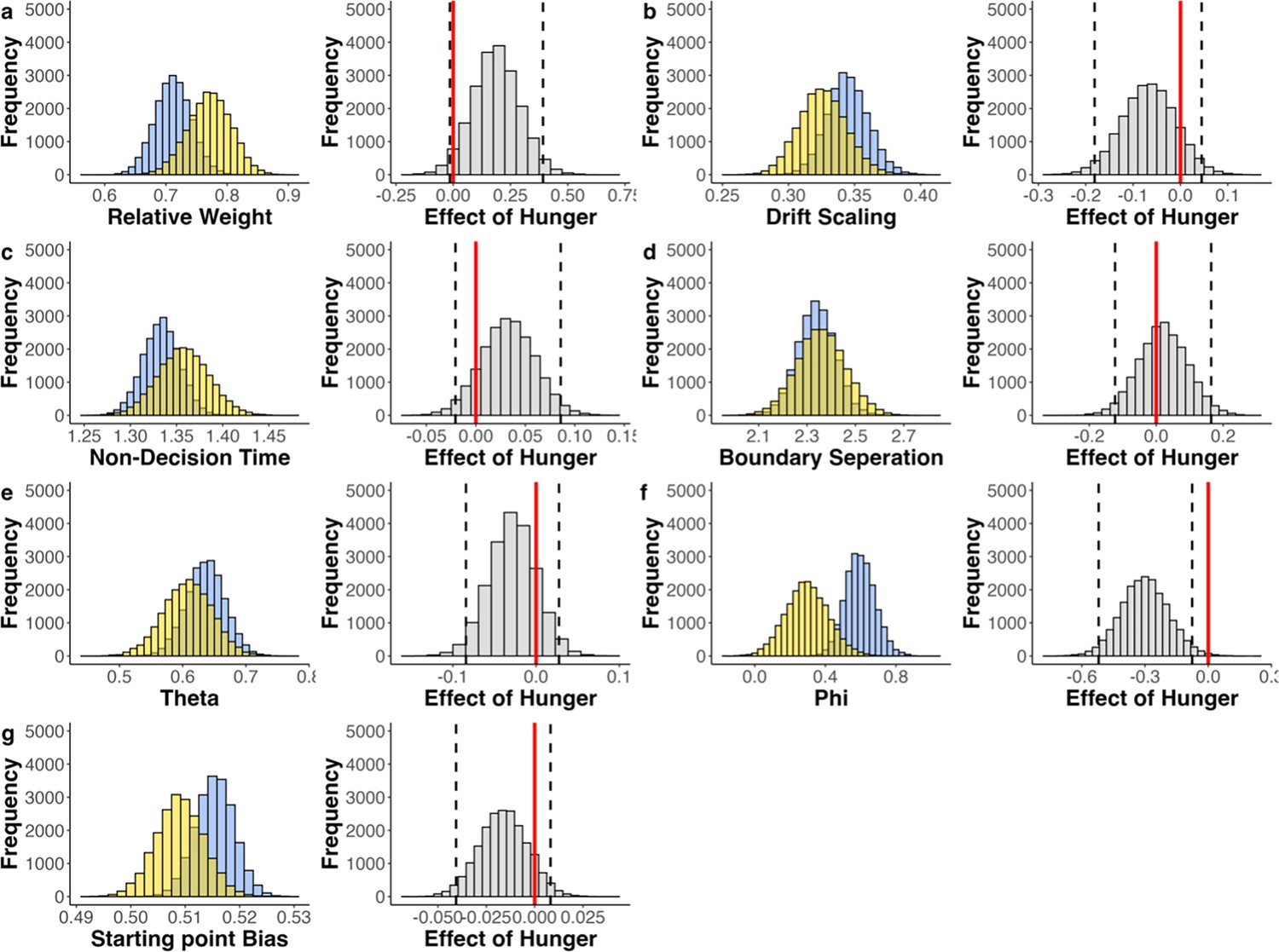
Fitted parameters of multi-attribute attentional DDM (maaDDM).

Fitted parameters across participants (blue = sated, yellow = hungry; left panels) and the effect of hunger state (gray; right panels). Dashed black lines indicate the 95% highest density interval (HDI) edges. If ‘0’ (red line) is included in HDI, no credible difference between conditions (a) Estimated relative taste weight across participants. In both conditions, the relative taste weight is larger than 0.5, indicating that participants generally weigh taste more than health. There is a positive shift in the distribution of this effect, and the HDI does not include 0, indicating that hungry individuals have a higher relative taste weight (**b–e**). Estimated parameter values for drift scaling, non-decision time (nDT), boundary separation, and theta across participants and the corresponding effects of hunger state. (f) Estimated parameter values for phi across participants. The corresponding effect of hunger indicates that hungry participants discount the non-looked upon attribute more strongly.

Figure 6

Download asset Open asset

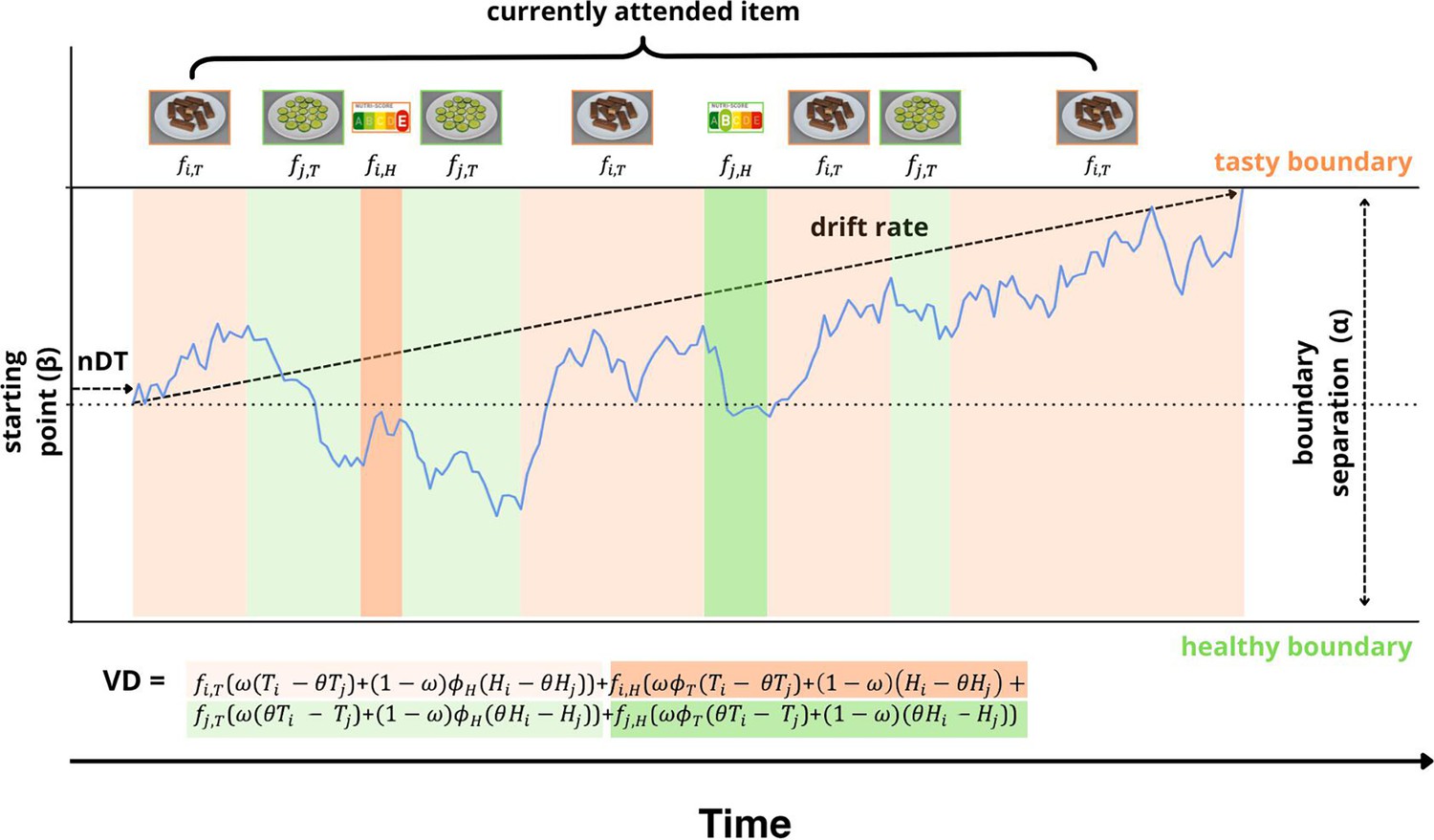
Illustration of the maaDDM2 $ϕ$ .

The decision-making process underlying choice and response time (RT) data as conceived by the *maaDDM2ϕ*. The decision is assumed to emerge from a noisy evidence-accumulation process commencing from the starting point ( $β$ ) and terminating at one of the two boundaries (here: 0=healthy boundary and $α$ = tasty boundary) representing the tasty and healthy choice, respectively. The non-decision time (nDT) reflects processes unrelated to the decision itself, here illustrated as stimulus encoding time. The drift rate represents the rate of evidence accumulation. It is determined by the scaled value difference (VD) of the displayed options, which in turn is given by the taste (T) and health (H) ratings of the options, the relative weight of tastiness $ω$ vs. healthiness (1- $ω$ ) as well as the currently attended item on the screen as illustrated by the differently colored segments and the corresponding images. The coloring scheme of the VD equation shows which part of the equation defines the drift rate at any given attended item. Attending to the tasty option (here: chocolate bar with Nutri-Score E), and in particular to its taste information (i.e. the image), increases the drift towards the tasty boundary (orange), while attending to the healthy option (here: cucumber with Nutri-Score B), and in particular to its health information (i.e. the Nutri-Score) increases the drift towards the healthy boundary (green).

Appendix 1—figure 1

Download asset Open asset

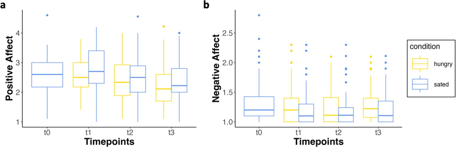
Mood across timepoints.

(a) Average positive affect (PA) scores across t; Welch-corrected RM-ANOVA of PA revealed a main effect of t (F(1.76, 119.43)=28.179, p<0.001, partial η²=0.046). and condition (F(1, 68)=5.013, p=0.028, partial η²=0.013): Bonferroni corrected post hoc comparisons demonstrated significant differences in PA between t1 and t3 in the hungry (p=0.007) and the sated condition (p=0.005), all other comparisons did not reach significance. (b) Average negative affect (NA) scores across timepoints (t). RM-ANOVA of NA revealed a main effect of condition; Bonferroni-corrected post hoc comparisons were not significant.

Appendix 2—figure 1

Download asset Open asset

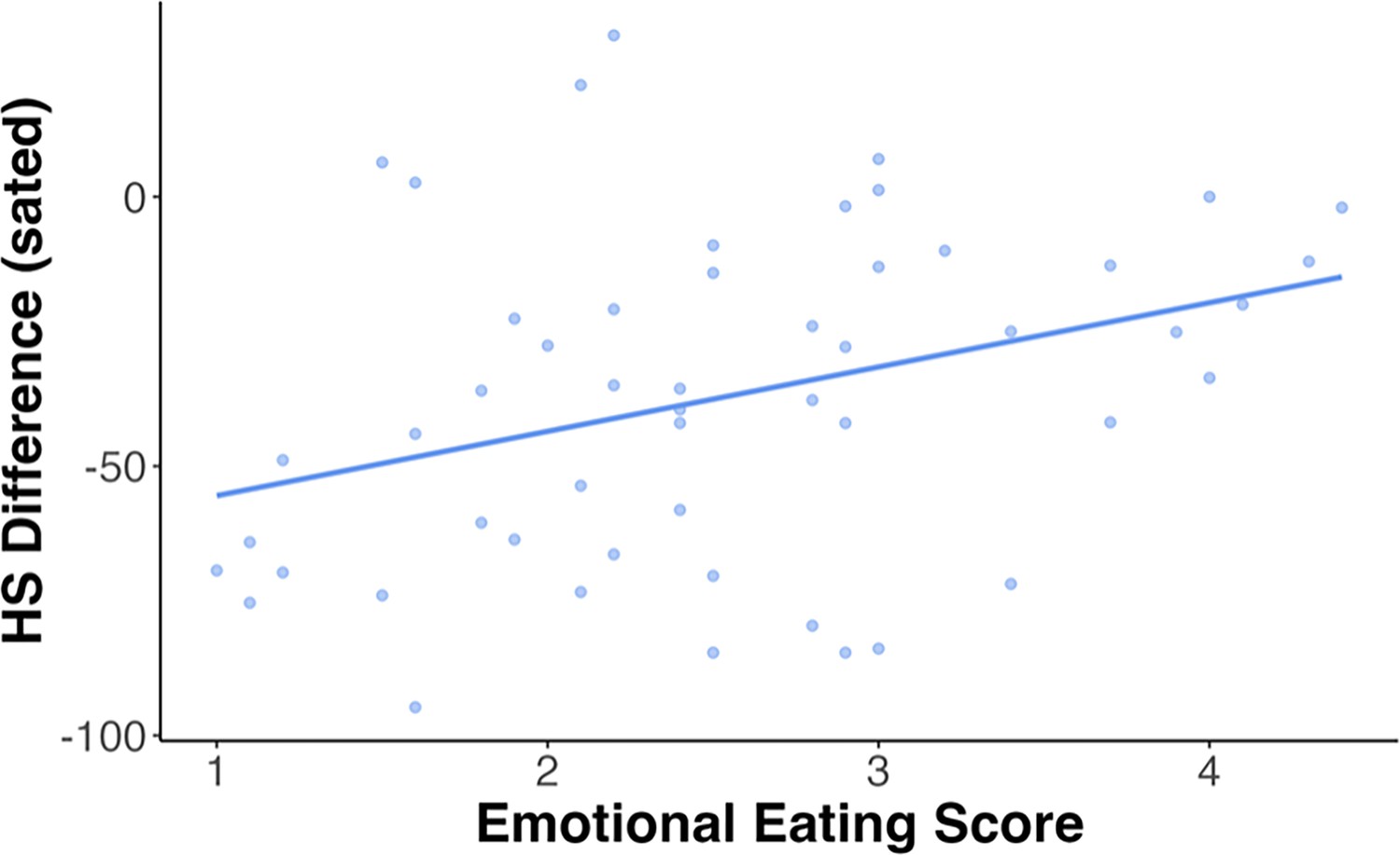
Correlations eating behavior and subjective hunger rating.

Individuals scoring higher on the subscale of emotional eating, report to be less sated by protein shake. A Pearson’s product-moment correlation revealed a moderate positive correlation between emotional eating and the difference in hunger ratings in the sated condition (r=0.34, *95% CI*=[0.08, 0.56], p=0.013, n=53). The other scales of the FEV did not yield any significant correlations with difference in hunger state (HS) across conditions and are, therefore, not shown here (see also *Table A2c*)

Appendix 3—figure 1

Download asset Open asset

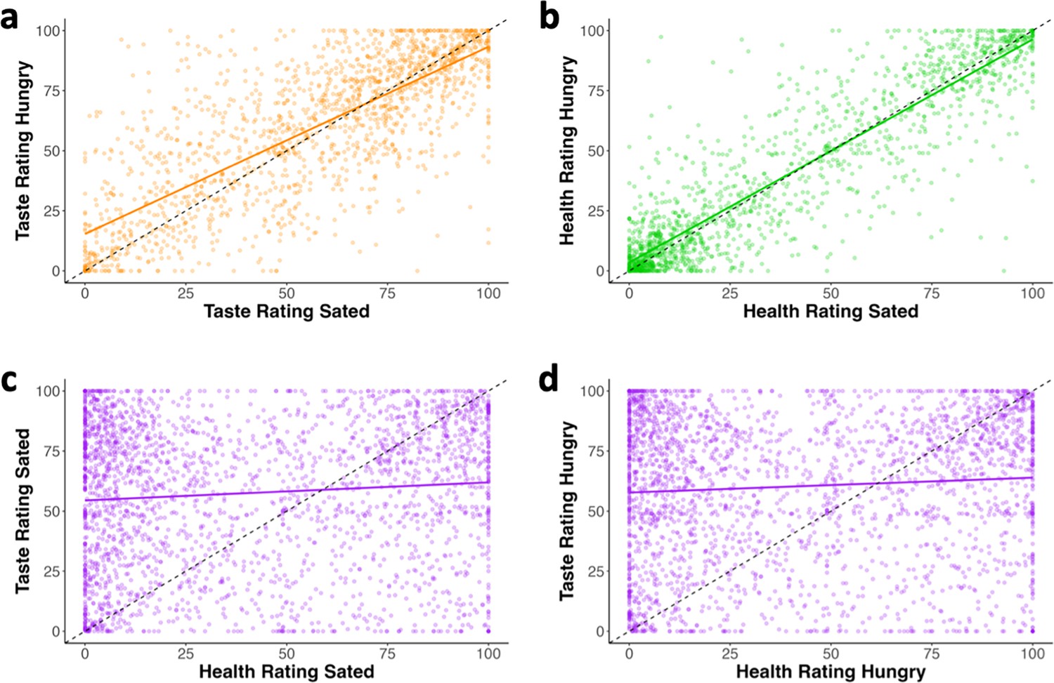
Correlation ratings across timepoints.

(a) Correlation taste across timepoints (t) (r=0.778), (b) Correlation health across t (r=0.916), (c) Correlation taste and health in the sated condition (r=0.316), (d) Correlation taste and health in the hungry condition (r=0.301).

Appendix 3—figure 2

Download asset Open asset

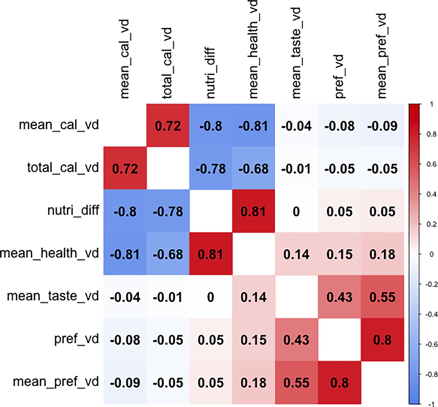
Correlations among predictors.

vd refers to value difference left – right option.

Appendix 8—figure 1

Download asset Open asset

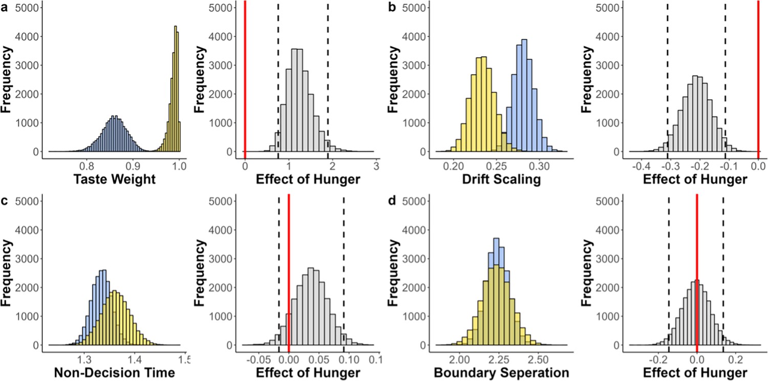
Fitted parameters of drift diffusion model (DDM).

Fitted parameters across participants (blue = sated, yellow = hungry; left panels) and the effect of hunger state (gray; right panels). Dashed black lines indicate the 95% highest density interval (HDI) edges. (a) Estimated relative taste weight across participants. In both conditions the relative taste weight is larger than 0.5, indicating that participants generally weigh taste more than health. There is a positive shift in the distribution of this effect, and the HDI does not include 0, indicating that hungry individuals have a higher relative taste weight (b) Estimated drift scaling across participants. There is a negative shift in the distribution of this effect, and the HDI does not include 0, which indicates that hungry individuals accumulate evidence less efficiently. Note, however, that the (better performing) multi-attribute attentional DDM (maaDDM) and maaDDM2f indicate that this effect is due to hunger-dependent attentional discounting. (**c, d**) Estimated parameter values for non-decision time (nDT) and boundary separation across participants and the corresponding effects of hunger state.

Appendix 8—figure 2

Download asset Open asset

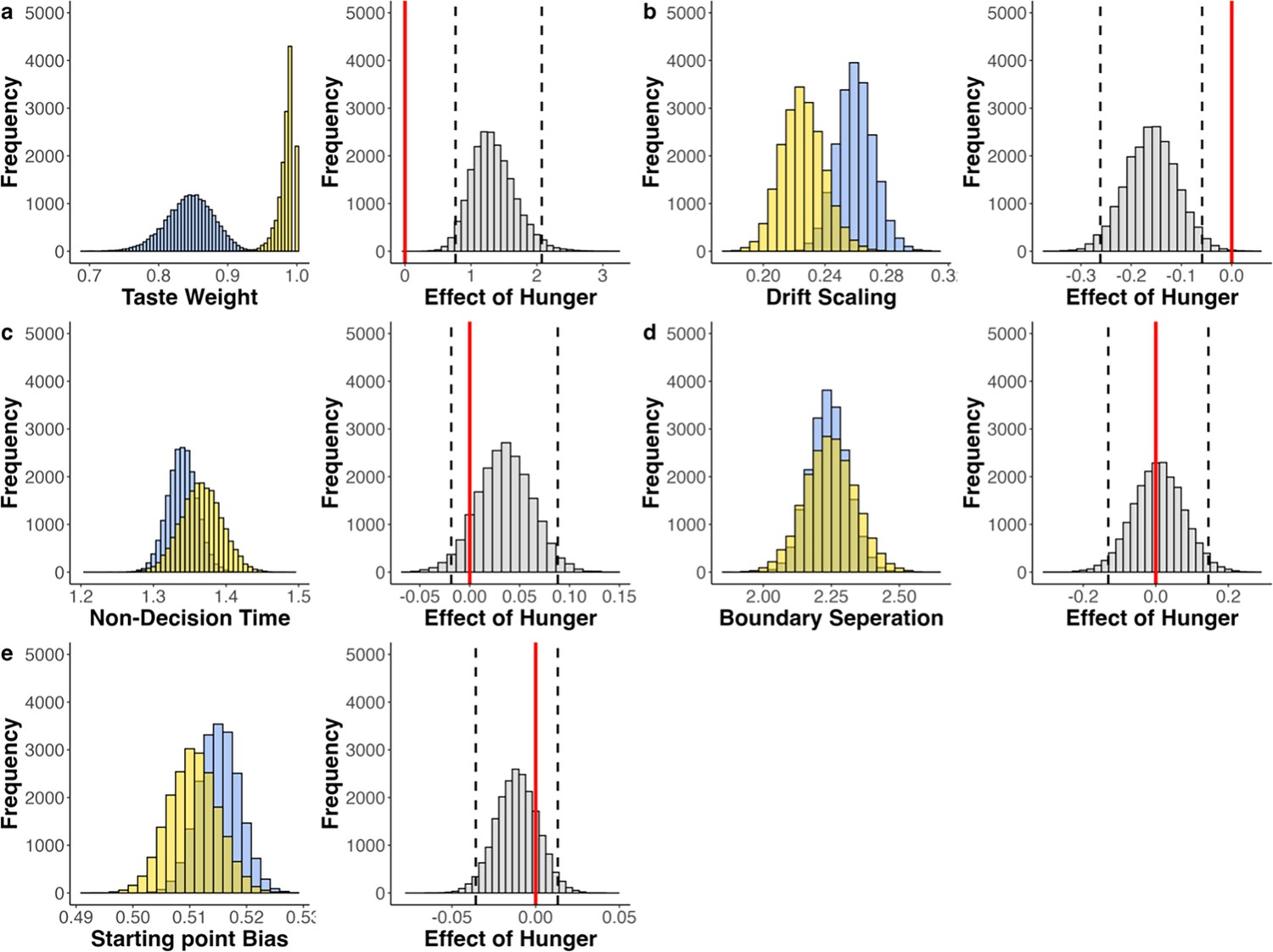
Fitted parameters of DDMsp.

Fitted parameters across participants (blue = sated, yellow = hungry; left panels) and the effect of hunger state (gray; right panels). Dashed black lines indicate the 95% highest density interval (HDI) edges. (a) Estimated relative taste weight across participants. In both conditions, the relative taste weight is larger than 0.5, indicating that participants generally weigh taste more than health. There is a positive shift in the distribution of this effect, and the HDI does not include 0, indicating that hungry individuals have a higher relative taste weight (b) Estimated drift scaling across participants. There is a negative shift in the distribution of this effect, and the HDI does not include 0, which indicates that hungry individuals accumulate evidence less efficiently. Note, however, that the (better performing) multi-attribute attentional DDM (maaDDM) and maaDDM2f indicate that this effect is due to hunger-dependent attentional discounting. (**c, d**) Estimated parameter values for non-decision time (nDT) and boundary separation across participants and the corresponding effects of hunger state. (e) Estimated parameter values for a relative starting point bias across participants and the corresponding effects of hunger state, indicating that sated individuals are biased towards the taste boundary (sated HDI does not include 0.5), but difference between conditions is not significant.

Appendix 8—figure 3

Download asset Open asset

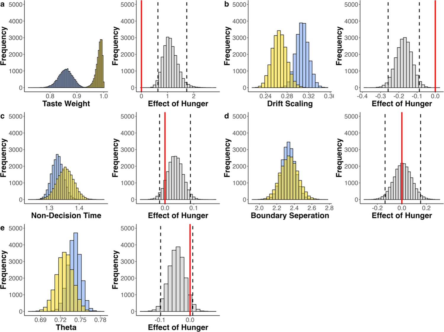
Fitted parameters of aDDM.

Fitted parameters across participants (blue = sated, yellow = hungry; left panels) and the effect of hunger state (gray; right panels). Dashed black lines indicate the 95% highest density interval (HDI) edges. (a) Estimated relative taste weight across participants. In both conditions, the relative taste weight is larger than 0.5, indicating that participants generally weigh taste more than health. There is a positive shift in the distribution of this effect, and the HDI does not include 0, indicating that hungry individuals have a higher relative taste weight (b) Estimated drift scaling across participants. There is a negative shift in the distribution of this effect, and the HDI does not include 0, which indicates that hungry individuals accumulate evidence less efficiently. Note, however, that the (better performing) multi-attribute attentional DDM (maaDDM) and maaDDM2f indicate that this effect is due to hunger-dependent attentional discounting. (**c-e**) Estimated parameter values for non-decision time (nDT), boundary separation, and theta across participants and the corresponding effects of hunger state.

Appendix 8—figure 4

Download asset Open asset

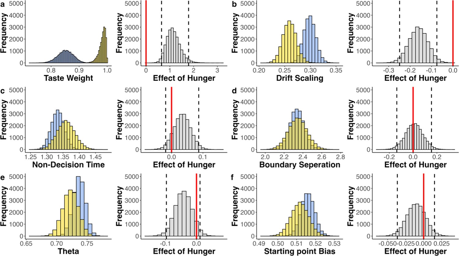
Fitted parameters of aDDMsp.

Fitted parameters across participants (blue = sated, yellow = hungry; left panels) and the effect of hunger state (gray; right panels). Dashed black lines indicate the 95% highest density interval (HDI) edges. If ‘0’ (red line) is included in HDI, no credible difference between conditions. (a) Estimated relative taste weight across participants. In both conditions, the relative taste weight is larger than 0.5, indicating that participants generally weigh taste more than health. There is a positive shift in the distribution of this effect, and the HDI does not include 0, indicating that hungry individuals have a higher relative taste weight (b) Estimated drift scaling across participants. There is a negative shift in the distribution of this effect, and the HDI does not include 0, which would indicate that hungry individuals accumulate evidence less efficiently. Note, however, that the (better performing) multi-attribute attentional DDM (maaDDM) and maaDDM2f indicate that this effect is due to hunger-dependent attentional discounting. (**c-e**) Estimated parameter values for non-decision time (nDT), boundary separation, and theta across participants and the corresponding effects of hunger state. (f) Estimated parameter values for a relative starting point bias across participants and the corresponding effects of hunger state, indicating that sated individuals are biased towards the taste boundary (sated HDI does not include 0.5), but difference between conditions is not significant.

Appendix 8—figure 5

Download asset Open asset

Fitted parameters of maaDDMsp.

Fitted parameters across participants (blue = sated, yellow = hungry; left panels) and the effect of hunger state (gray; right panels). Dashed black lines indicate the 95% highest density interval (HDI) edges. If ‘0’ (red line) is included in HDI, no credible difference between conditions. (a) Estimated relative taste weight across participants. In both conditions, the relative taste weight is larger than 0.5, indicating that participants generally weigh taste more than health. There is a positive shift in the distribution of this effect, and the HDI does not include 0, indicating that hungry individuals have a higher relative taste weight (**b-e**). Estimated parameter values for drift scaling, non-decision time (nDT), boundary separation, and theta across participants and the corresponding effects of hunger state. (f) Estimated parameter values for phi across participants. The corresponding effect of hunger indicates that hungry participants discount the non-looked upon attribute more strongly (g). Estimated parameter values for a relative starting point bias across participants and the corresponding effects of hunger state indicate that sated individuals are biased towards the taste boundary (sated HDI does not include 0.5), but difference between conditions is not significant.

Appendix 8—figure 6

Download asset Open asset

Fitted parameters of maaDDM2 $ϕ$ sp.

Fitted parameters across participants (blue = sated, yellow = hungry; left panels) and the effect of hunger state (gray; right panels). Dashed black lines indicate the 95% highest density interval (HDI) edges. If ‘0’ (red line) is included in HDI, no credible difference between conditions. (a) Estimated relative taste weight across participants. In both conditions, the relative taste weight is larger than 0.5, indicating that participants generally weigh taste more than health. There is a marginal positive shift in the distribution of this effect, indicating that hungry individuals have a higher relative taste weight (**b-d**). Estimated parameter values for drift scaling, non-decision time (nDT), boundary and separation across participants and the corresponding effects of hunger state. (e) Estimated parameter values for a relative starting point bias across participants and the corresponding effects of hunger state, indicating that sated individuals are biased. towards the taste boundary (sated HDI does not include 0.5), but difference between conditions is not significant. (f) Estimated parameter values for theta across participants and the corresponding effects of hunger state. (g) Estimated parameter values for $ϕ_{T}$ and the corresponding effects of hunger state. (h) Parameter estimates of $ϕ_{H}$ and the corresponding effects of hunger state, showing that the attention-driven discounting of health information was amplified under hunger.

Appendix 9—figure 1

Download asset Open asset

Posterior predictive checks maaDDMsp and maaDDM2 $ϕ$ sp.

Quantile plots of simulated data with fitted parameters of (a) the *maaDDMsp* and (b) the *maaDDM2* $ϕ$ sp in blue (sated) and yellow (hungry) with highest density intervals (HDIs) of each quantile (vertical lines) and behavior.

Appendix 10—figure 1

Download asset Open asset

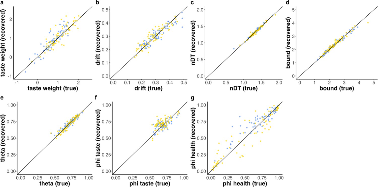
Parameter recovery maaDDM2 $ϕ$ .

We generated data based on the means of each parameter and simulated 70 datasets with 180 trials each using empirical subjective value-ratings and gaze patterns. (a) The correlation between true and recovered weight parameter was r=0.924 in the sated (blue), and r=0.913 in the hungry (yellow) condition. (b) The correlation between true and recovered drift scaling parameter was r=0.921 in the sated (blue), and r=0.91 in the hungry (yellow) condition. (c) The correlation between true and recovered non-decision time parameter was r=0.984 in the sated (blue), and r=0.986 in the hungry (yellow) condition. (d) The correlation between true and recovered boundary separation parameter was r=0.989 in the sated (blue), and r=0.982 in the hungry (yellow) condition. (e) The correlation between true and recovered theta parameter was r=0.937 in the sated (blue), and r=0.953 in the hungry (yellow) condition. (f) The correlation between true and recovered taste phi parameter was r=0.704 in the sated (blue), and r=0.712 in the hungry (yellow) condition. (g) The correlation between true and recovered health phi parameter was r=0.928 in the sated (blue), and r=0.94 in the hungry (yellow) condition.

Appendix 10—figure 2

Download asset Open asset

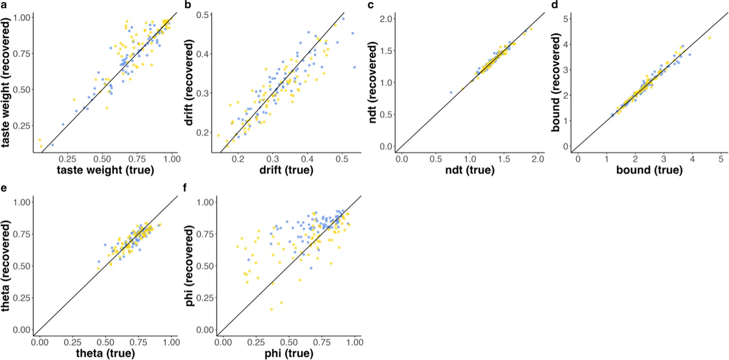
Parameter recovery multi-attribute attentional DDM (maaDDM).

We generated data based on the means of each parameter and simulated 70 datasets with 180 trials each using empirical subjective value-ratings and gaze patterns. (a) The correlation between true and recovered taste weight parameter was r=0.914 in the sated (blue), and r=0.867 in the hungry (yellow) condition. (b) The correlation between true and recovered drift scaling parameter was r=0.902 in the sated (blue), and r=0.875 in the hungry (yellow) condition. (c) The correlation between true and recovered non-decision time parameter was r=0.976 in the sated (blue), and r=0. 985 in the hungry (yellow) condition. (d) The correlation between true and recovered boundary separation parameter was r=0.983 in the sated (blue), and r=0.985 in the hungry (yellow) condition. (e) The correlation between true and recovered theta parameter was r=0.799 in the sated (blue), and r=0.872 in the hungry (yellow) condition. (f) The correlation between true and recovered phi parameter was r=0.615 in the sated (blue), and r=0.618 in the hungry (yellow) condition.

Appendix 10—figure 3

Download asset Open asset

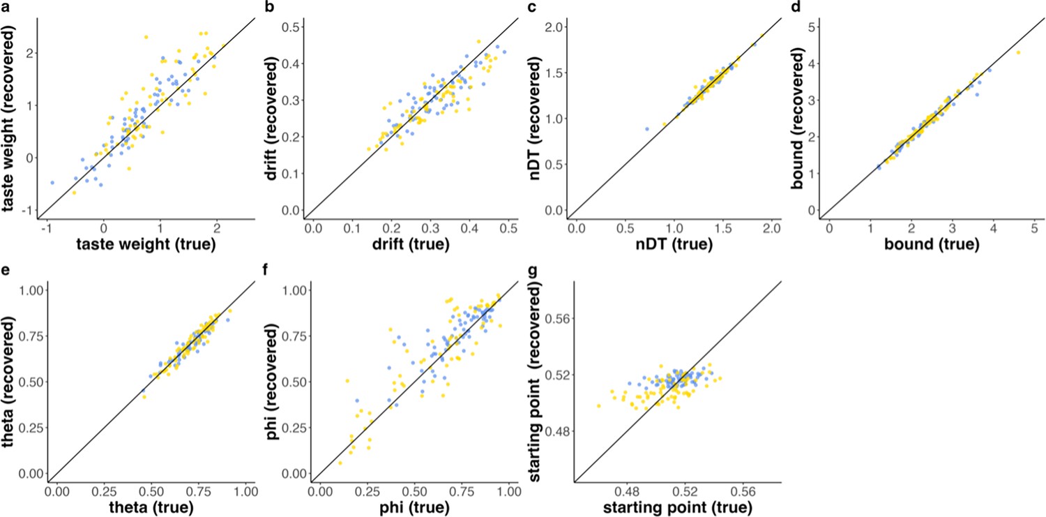
Parameter recovery maaDDMsp.

We generated data based on the means of each parameter and simulated 70 datasets with 180 trials each using empirical subjective value-ratings and gaze patterns. (a) The correlation between true and recovered relative taste weight parameter was r=0.936 in the sated (blue), and r=0.888 in the hungry (yellow) condition. (b) The correlation between true and recovered drift scaling parameter was r=0.876 in the sated (blue), and r=0.885 in the hungry (yellow) condition. (c) The correlation between true and recovered non-decision time parameter was r=0.977 in the sated (blue), and r=0.984 in the hungry (yellow) condition. (d) The correlation between true and recovered boundary separation parameter was r=0.988 in the sated (blue), and r=0.99 in the hungry (yellow) condition. (e) The correlation between true and recovered theta parameter was r=0.943 in the sated (blue), and r=0.962 in the hungry (yellow) condition. (f) The correlation between true and recovered phi parameter was r=0.863 in the sated (blue), and r=0.864 in the hungry (yellow) condition. (g) The correlation between true and recovered starting point bias parameter was r=0.417 in the sated (blue), and r=0.577 in the hungry (yellow) condition.

Appendix 10—figure 4

Download asset Open asset

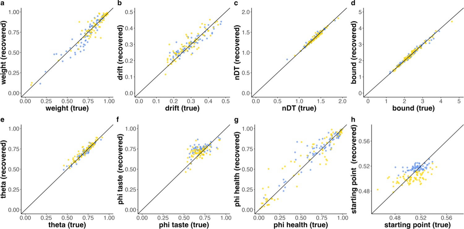
Parameter recovery maaDDM2 $ϕ$ sp.

We generated data based on the means of each parameter and simulated 70 datasets with 180 trials each using empirical subjective value-ratings and gaze patterns. (a) The correlation between true and recovered weight parameter was r=0.938 in the sated (blue), and r=0.915 in the hungry (yellow) condition. (b) The correlation between true and recovered drift scaling parameter was r=0.912 in the sated (blue), and r=0.892 in the hungry (yellow) condition. (c) The correlation between true and recovered non-decision time parameter was r=0.982 in the sated (blue), and r=0.984 in the hungry (yellow) condition. (d) The correlation between true and recovered boundary separation parameter was r=0.99 in the sated (blue), and r=0.989 in the hungry (yellow) condition. (e) The correlation between true and recovered theta parameter was r=0.956 in the sated (blue), and r=0.947 in the hungry (yellow) condition. (f) The correlation between true and recovered taste phi parameter was r=0.594 in the sated (blue), and r=0.593 in the hungry (yellow) condition. (g) The correlation between true and recovered health phi parameter was r=0.921 in the sated (blue), and r=0.939 in the hungry (yellow) condition. (h) The correlation between true and recovered starting point bias parameter was r=0.521 in the sated (blue), and r=0.62 in the hungry (yellow) condition.

Appendix 11—figure 1

Download asset Open asset

Fitted parameters of DDM of models with Nutri-Score reflecting health value.

Fitted parameters across participants (blue = sated, yellow = hungry; left panels) and the effect of hunger state (gray; right panels). Dashed black lines indicate the 95% highest density interval (HDI) edges. (a) Estimated relative taste weight across participants. In both conditions, the relative taste weight is larger than 0.5, indicating that participants generally weigh taste more than health. There is a positive shift in the distribution of this effect, and the HDI does not include 0, indicating that hungry individuals have a higher relative taste weight (b) Estimated drift scaling across participants. There is a negative shift in the distribution of this effect, and the HDI does not include 0, which indicates that hungry individuals accumulate evidence less efficiently. Note, however, that the (better performing) multi-attribute attentional DDM (maaDDM) and maaDDM2f indicate that this effect is due to hunger-dependent attentional discounting. (**c, d**) Estimated parameter values for non-decision time (nDT) and boundary separation across participants and the corresponding effects of hunger state.

Appendix 11—figure 2

Download asset Open asset

Fitted parameters of DDMsp of models with Nutri-Score reflecting health value.

Fitted parameters across participants (blue = sated, yellow = hungry; left panels) and the effect of hunger state (gray; right panels). Dashed black lines indicate the 95% highest density interval (HDI) edges. (a) Estimated relative taste weight across participants. In both conditions, the relative taste weight is larger than 0.5, indicating that participants generally weigh taste more than health. There is a positive shift in the distribution of this effect, and the HDI does not include 0, indicating that hungry individuals have a higher relative taste weight (b) Estimated drift scaling across participants. There is a negative shift in the distribution of this effect, and the HDI does not include 0, which indicates that hungry individuals accumulate evidence less efficiently. Note, however, that the (better performing) multi-attribute attentional DDM (maaDDM) and maaDDM2f indicate that this effect is due to hunger-dependent attentional discounting. (**c, d**) Estimated parameter values for non-decision time (nDT) and boundary separation across participants and the corresponding effects of hunger state. (e) Estimated parameter values for a relative starting point bias across participants and the corresponding effects of hunger state, indicating that sated individuals are biased towards the taste boundary (sated HDI does not include 0.5), but difference between conditions is not significant.

Appendix 11—figure 3

Download asset Open asset

Fitted parameters of aDDM of models with Nutri-Score reflecting health value.

Fitted Parameters across participants (blue = sated, yellow = hungry; left panels) and the effect of hunger state (gray; right panels). Dashed black lines indicate the 95% highest density interval (HDI edges). (a) Estimated relative taste weight across participants. In both conditions, the relative taste weight is larger than 0.5, indicating that participants generally weigh taste more than health. There is a positive shift in the distribution of this effect, and the HDI does not include 0, indicating that hungry individuals have a higher relative taste weight (b) Estimated drift scaling across participants. There is a negative shift in the distribution of this effect, and the HDI does not include 0, which indicates that hungry individuals accumulate evidence less efficiently. Note, however, that the (better performing) multi-attribute attentional DDM (maaDDM) and maaDDM2f indicate that this effect is due to hunger-dependent attentional discounting. (**c-e**) Estimated parameter values for non-decision time (nDT), boundary separation, and theta across participants and the corresponding effects of hunger state.

Appendix 11—figure 4

Download asset Open asset

Fitted parameters of aDDMsp of models with nutri-score reflecting health value.

Fitted parameters across participants (blue = sated, yellow = hungry; left panels) and the effect of hunger state (gray; right panels). Dashed black lines indicate the 95% highest density interval (HDI) edges. If ‘0’ (red line) is included in HDI, no credible difference between conditions. (a) Estimated relative taste weight across participants. In both conditions, the relative taste weight is larger than 0.5, indicating that participants generally weigh taste more than health. There is a positive shift in the distribution of this effect, and the HDI does not include 0, indicating that hungry individuals have a higher relative taste weight (b) Estimated drift scaling across participants. There is a negative shift in the distribution of this effect, and the HDI does not include 0, which would indicate that hungry individuals accumulate evidence less efficiently. Note, however, that the (better performing) multi-attribute attentional DDM (maaDDM) and maaDDM2f indicate that this effect is due to hunger-dependent attentional discounting. (**c-e**) Estimated parameter values for non-decision time (nDT), boundary separation, and theta across participants and the corresponding effects of hunger state. (f) Estimated parameter values for a relative starting point bias across participants and the corresponding effects of hunger state, indicating that sated individuals are biased towards the taste boundary (sated HDI does not include 0.5), but difference between conditions is not significant.

Appendix 11—figure 5

Download asset Open asset

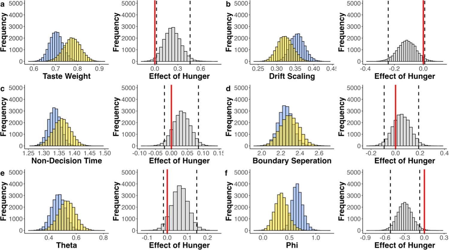
Fitted parameters of multi-attribute attentional DDM (maaDDM) of models with nutri-score reflecting health value.

Fitted parameters across participants (blue = sated, yellow = hungry; left panels) and the effect of hunger state (gray; right panels). Dashed black lines indicate the 95% highest density interval (HDI) edges. If ‘0’ (red line) is included in HDI, no credible difference between conditions (a) Estimated relative taste weight across participants. In both conditions, the relative taste weight is larger than 0.5, indicating that participants generally weigh taste more than health. There is a positive shift in the distribution of this effect, and the HDI does not include 0, indicating that hungry individuals have a higher relative taste weight (**b-e**). Estimated parameter values for drift scaling, non-decision time (nDT), boundary separation, and theta across participants and the corresponding effects of hunger state. (f) Estimated parameter values for phi across participants. The corresponding effect of hunger indicates that hungry participants discount the non-looked-upon attribute more strongly.

Appendix 11—figure 6

Download asset Open asset

Fitted parameters of maaDDMsp of models with nutri-score reflecting health value.

Fitted parameters across participants (blue = sated, yellow = hungry; left panels) and the effect of hunger state (gray; right panels). Dashed black lines indicate the 95% highest density interval (HDI) edges. If ‘0’ (red line) is included in HDI, no credible difference between conditions. (a) Estimated relative taste weight across participants. In both conditions the relative taste weight is larger than 0.5, indicating that participants generally weigh taste more than health. There is a positive shift in the distribution of this effect, and the HDI does not include 0, indicating that hungry individuals have a higher relative taste weight (**b-e**). Estimated parameter values for drift scaling, non-decision time (nDT), boundary separation, and theta across participants and the corresponding effects of hunger state. (f) Estimated parameter values for phi across participants. The corresponding effect of hunger indicates that hungry participants discount the non-looked upon attribute more strongly (g). Estimated parameter values for a relative starting point bias across participants and the corresponding effects of hunger state indicate that sated individuals are biased towards the taste boundary (sated HDI does not include 5), but difference between conditions is not significant.

Appendix 11—figure 7

Download asset Open asset

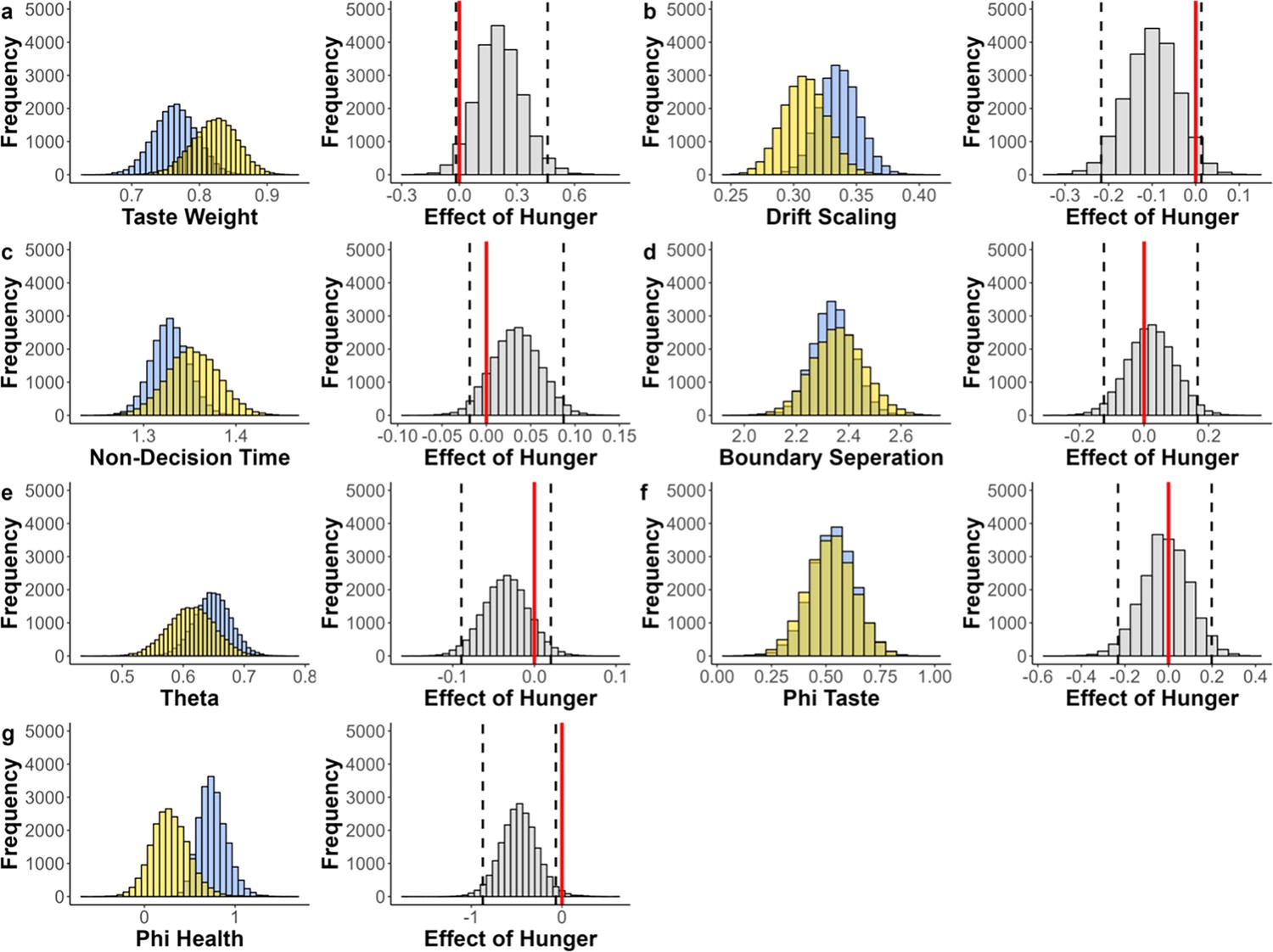
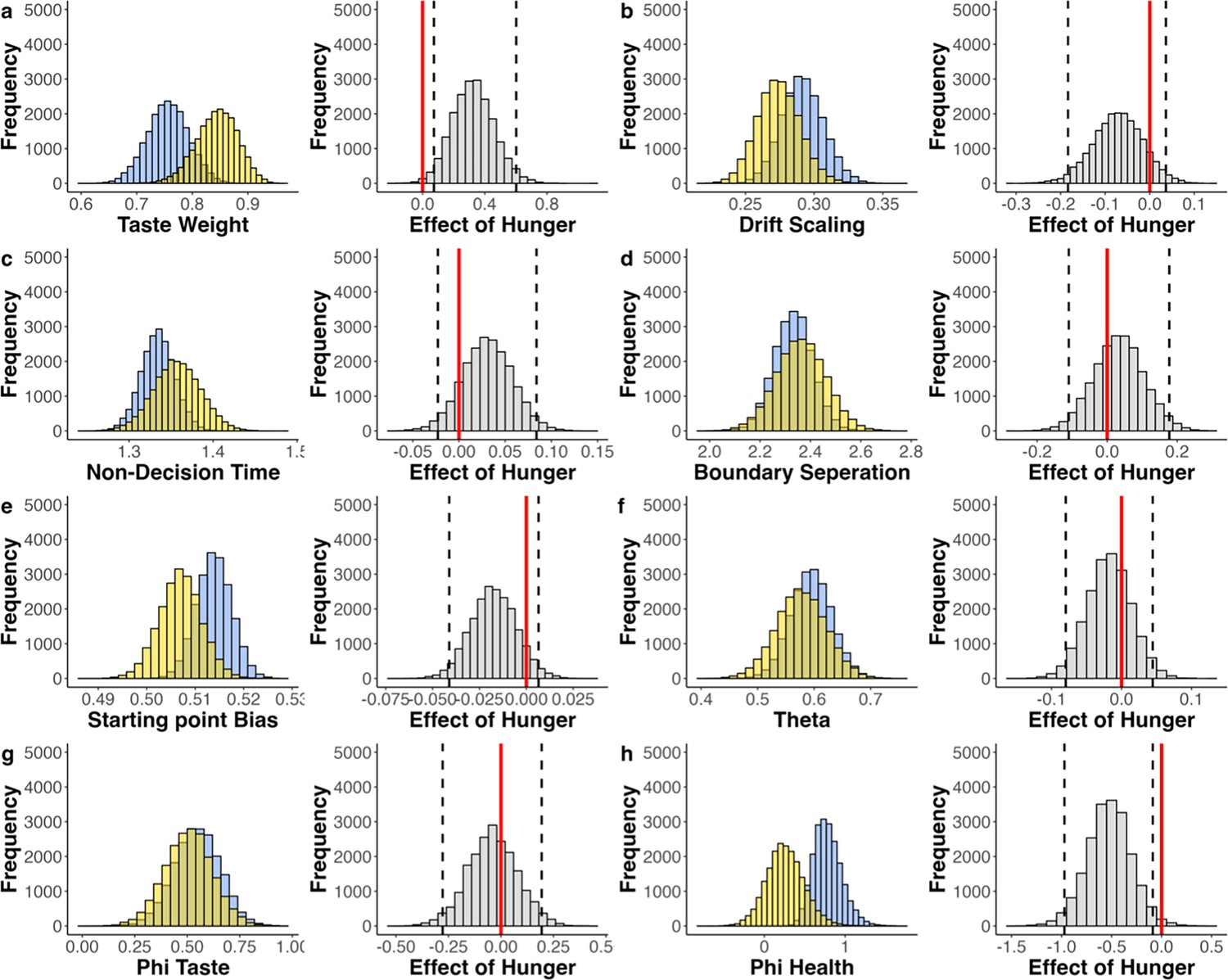
Fitted parameters of maaDDM2 $ϕ$ of models with Nutri-Score reflecting health value.

Fitted parameters across participants (blue = sated, yellow = hungry; left panels) and the effect of hunger state (gray; right panels). Dashed black lines indicate the 95% highest density interval (HDI) edges. If ‘0’ (red line) is included in HDI, no credible difference between conditions. (a) Estimated relative taste weight across participants. In both conditions, the relative taste weight is larger than 0.5, indicating that participants generally weigh taste more than Nutri-Score. There is a marginal positive shift in the distribution of this effect, indicating that hungry individuals have a higher relative taste weight (**b–f**). Estimated parameter values for $d$ , nDT, $α$ , $θ$ , and $ϕ_{T}$ across participants and the corresponding effects of hunger state. (g) Parameter estimates of $ϕ_{H}$ and the corresponding effects of hunger state, showing that the attention-driven discounting of health information was amplified under hunger.

Appendix 11—figure 8

Download asset Open asset

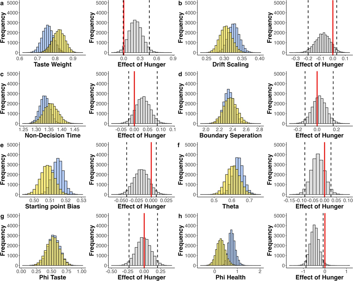
Fitted parameters of maaDDM2 $ϕ$ sp of Models with Nutri-Score reflecting health value.

Fitted parameters across participants (blue = sated, yellow = hungry; left panels) and the effect of hunger state (gray; right panels). Dashed black lines indicate the 95% highest density interval (HDI) edges. If ‘0’ (red line) is included in HDI, no credible difference between conditions. (a) Estimated relative taste weight across participants. In both conditions, the relative taste weight is larger than 0.5, indicating that participants generally weigh taste more than Nutri-Score. There is a marginal positive shift in the distribution of this effect, indicating that hungry individuals have a higher relative taste weight (**b-d**). Estimated parameter values for drift scaling, non-decision time (nDT), boundary and separation across participants and the corresponding effects of hunger state. (e) Estimated parameter values for a relative starting point bias across participants and the corresponding effects of hunger state, indicating that sated individuals are biased towards the taste boundary (sated HDI does not include 0.5), but difference between conditions is not significant. (f) Estimated parameter values for theta across participants and the corresponding effects of hunger state. (g) Estimated parameter values for $ϕ_{T}$ and the corresponding effects of hunger state. (h) Parameter estimates of $ϕ_{H}$ and the corresponding effects of hunger state, showing that the attention-driven discounting of health information was amplified under hunger.

Appendix 12—figure 1

Download asset Open asset

Fitted parameters of maaDDM of models with wanting reflecting taste value.

Fitted parameters across participants (blue = sated, yellow = hungry; left panels) and the effect of hunger state (gray; right panels). Dashed black lines indicate the 95% highest density interval (HDI) edges. If ‘0’ (red line) is included in HDI, no credible difference between conditions (a) Estimated relative taste weight across participants. In both conditions, the relative taste weight is larger than 0.5, indicating that participants generally weigh taste more than health. There is a positive shift in the distribution of this effect, and the HDI does not include 0, indicating that hungry individuals have a higher relative taste weight (**b-e**). Estimated parameter values for drift scaling, non-decision time (nDT), boundary separation, and theta across participants and the corresponding effects of hunger state. (f) Estimated parameter values for phi across participants. The corresponding effect of hunger indicates that hungry participants discount the non-looked upon attribute more strongly.

Appendix 12—figure 2

Download asset Open asset

Fitted parameters of maaDDM of models with wanting reflecting taste value and Nutri-Score reflecting health value.

Fitted parameters across participants (blue = sated, yellow = hungry; left panels) and the effect of hunger state (gray; right panels). Dashed black lines indicate the 95% highest density interval (HDI) edges. If ‘0’ (red line) is included in HDI, no credible difference between conditions (a) Estimated relative taste weight across participants. In both conditions, the relative taste weight is larger than 0.5, indicating that participants generally weigh taste more than health. There is a positive shift in the distribution of this effect, and the HDI does not include 0, indicating that hungry individuals have a higher relative taste weight (**b-e**). Estimated parameter values for drift scaling, non-decision time (nDT), boundary separation, and theta across participants and the corresponding effects of hunger state. (f) Estimated parameter values for phi across participants. The corresponding effect of hunger indicates that hungry participants discount the non-looked upon attribute more strongly.

Appendix 12—figure 3

Download asset Open asset

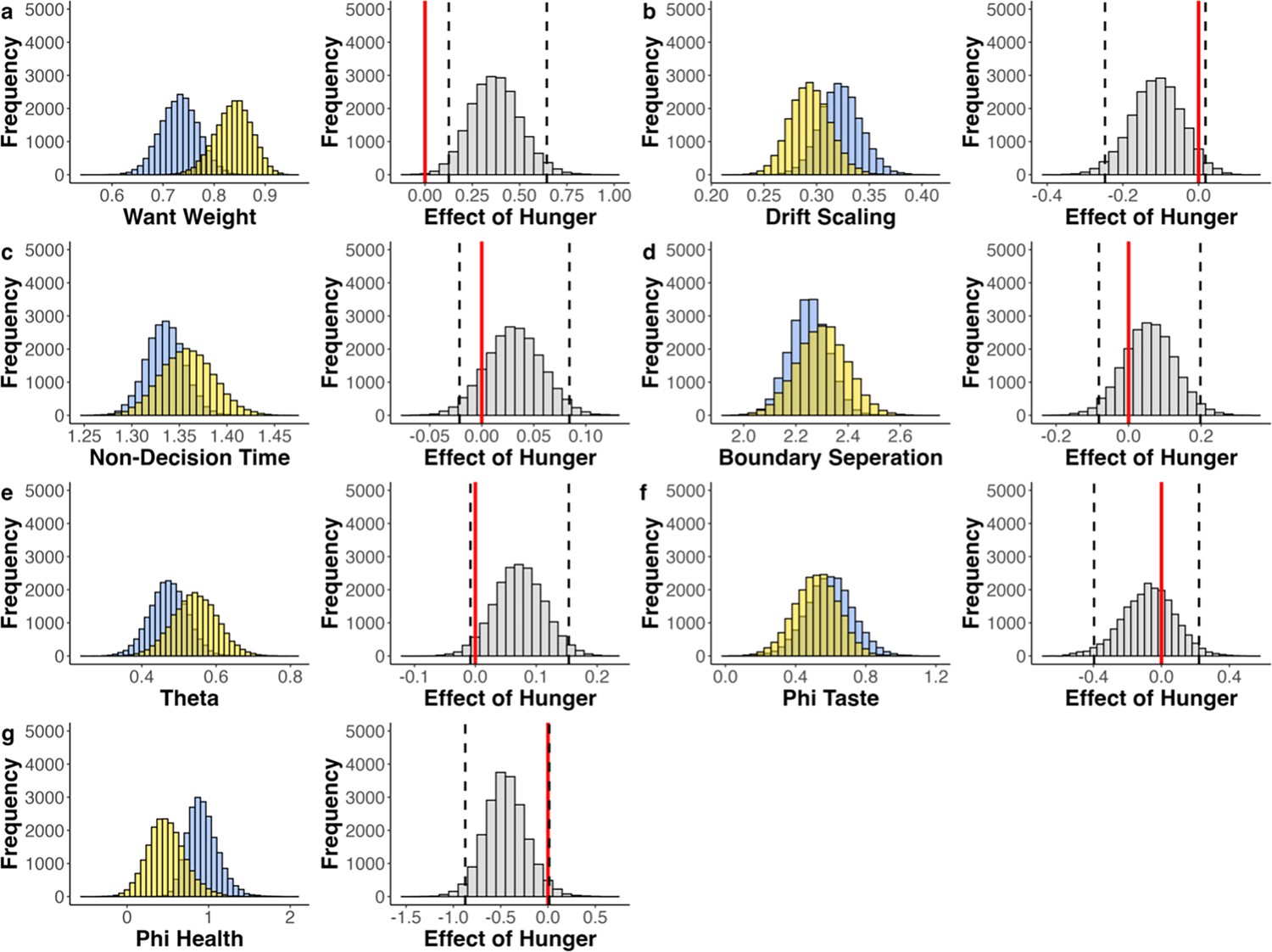
Fitted parameters of maaDDM2 $ϕ$ of models with wanting reflecting taste value.

Fitted parameters across participants (blue = sated, yellow = hungry; left panels) and the effect of hunger state (gray; right panels). Dashed black lines indicate the 95% highest density interval (HDI) edges. If ‘0’ (red line) is included in HDI, no credible difference between conditions. (a) Estimated relative taste weight across participants. In both conditions, the relative taste weight is larger than 0.5, indicating that participants generally weigh taste more than health. There is a positive shift in the distribution of this effect, and the HDI does not include 0, indicating that hungry individuals have a higher relative taste weight (**b-f**). Estimated parameter values for $d$ , nDT, $α$ , $θ$ , and $ϕ_{T}$ n across participants and the corresponding effects of hunger state. (g) Parameter estimates of $ϕ_{H}$ and the corresponding effects of hunger state, showing that the attention-driven discounting of health information was amplified under hunger.

Appendix 12—figure 4

Download asset Open asset

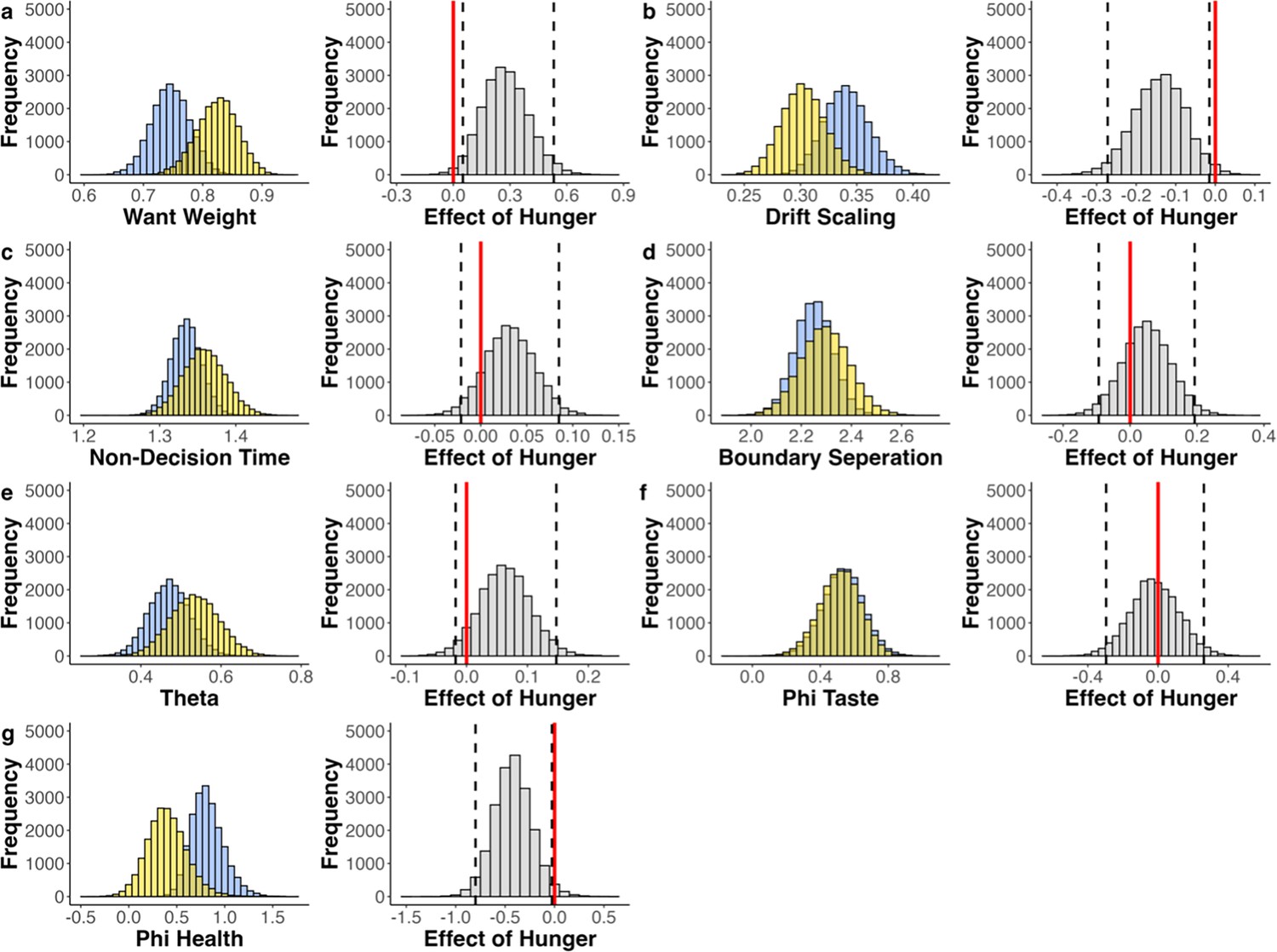
Fitted Parameters of maaDDM2 $ϕ$ of Models with Wanting Reflecting Taste Value and Nutri-Score Reflecting Health Value.

Fitted parameters across participants (blue = sated, yellow = hungry; left panels) and the effect of hunger state (gray; right panels). Dashed black lines indicate the 95% highest density interval (HDI) edges. If ‘0’ (red line) is included in HDI, no credible difference between conditions. (a) Estimated relative taste weight across participants. In both conditions, the relative taste weight is larger than 0.5, indicating that participants generally weigh taste more than health. There is a positive shift in the distribution of this effect, and the HDI does not include 0, indicating that hungry individuals have a higher relative taste weight (b) Estimated drift scaling across participants. There is a negative shift in the distribution of this effect, and the HDI does not include 0, which indicates that hungry individuals accumulate evidence less efficiently (**c-f**). Estimated parameter values for nDT, $α$ , $θ$ , and $ϕ_{T}$ n across participants and the corresponding effects of hunger state. (g) Parameter estimates of $ϕ_{H}$ and the corresponding effects of hunger state, showing that the attention-driven discounting of health information was amplified under hunger.

Author response image 1

Download asset Open asset

Author response image 2

Download asset Open asset

Author response image 3

Download asset Open asset

Author response image 4

Download asset Open asset

Author response image 5

Download asset Open asset

Tables

Table 1

Quantitative model comparison.

Model	$α$	nDT	$d$	$ω$	$β$	$θ$	$ϕ_{1}$	$ϕ_{2}$	DIC	Rhat
DDM	YES	YES	YES	YES	NO	NO	NO	NO	69646	1.002
DDMsp	YES	YES	YES	YES	YES	NO	NO	NO	69668	1.004
aDDM	YES	YES	YES	YES	NO	YES	NO	NO	65561	1.004
aDDMsp	YES	YES	YES	YES	YES	YES	NO	NO	65587	1.003
maaDDM	YES	YES	YES	YES	NO	YES	YES	NO	65155	1.005
maaDDMsp	YES	YES	YES	YES	YES	YES	YES	NO	65214	1.011
maaDDM2 ɸ	YES	YES	YES	YES	NO	YES	YES	YES	64002	1.017
maaDDM2 $ϕ$ sp	YES	YES	YES	YES	YES	YES	YES	YES	65070	1.027

The first column states the name of the model; the following nine columns indicate whether the drift diffusion model (DDM) variants included a given parameter or not. $α$ refers to the boundary separation; nDT refers to non-decision time; $d$ refers to the drift scaling parameter; $ω$ refers to the relative taste compared to health weight; $β$ refers to the starting point bias; $θ$ refers to the discounting of the non-looked upon option; $ϕ_{1}$ refers to the discounting of the non-looked upon attribute, in case the model includes $ϕ_{1}$ and $ϕ_{2}$ they refer to the discounting of taste and heath information, respectively; The deviance information criterion (DIC) was used as goodness-of-fit measure. Rhat is the scale reduction factor, to accurately predict posterior distributions, it should be 1.00, according to Vuorre and Bolger, 2018 values within 0.05 are acceptable. The best model (i.e. maaDDM2 $ϕ$ ) is highlighted in bold.

Appendix 4—table 1

Effect of hunger state on tasty vs healthy choice.

a) GLMM 1: Results of tasty choice given condition and attention*
	Fixed effects
	Estimate	Std. Error	z value	Pr(>\|z\|)
(Intercept)	0.832	0.102	8.164	<0.001***
conditionsated	–0.211	0.103	–2.05	0.04*
rel_DT_tasty_option	0.998	0.027	36.363	<0.001***
	Random Effects
	Variance	S. D.	Correlation
Subject (Intercept)	0.635	0.797
conditionsated \| subject	0.57	0.755	–0.59
b) GLMM 2: Results of tasty choice given condition, attention, and additional predictors 1^†
	Fixed effects
	Estimate	Std. Error	z value	Pr(>\|z\|)
(Intercept)	0.817	0.1	8.297	<0.001***
conditionsated	–0.19	0.096	–1.94	0.052
rel_DT_tasty_option	0.999	0.027	36.331	<0.001***
rel_dwelldiff_food	0.093	0.028	3.267	0.001**
BMI_cent	0.015	0.019	0.774	0.439
age_cent	–0.023	0.013	–1.798	0.072
conditionsated * age_cent	0.022	0.012	1.8	0.072
rel_DT_tasty_option * BMI_cent	–0.017	0.009	–1.913	0.056
rel_DT_tasty_option * age_cent	–0.011	0.004	–2.645	0.008**
	Random effects
	Variance	S. D.	Correlation
Subject (Intercept)	0.601	0.776
Conditionsated \| subject	0.498	0.706	–0.59
c) GLMM 3: Results of tasty choice given condition, attention and additional predictors 2 ^‡
	Estimate	Std. Error	z value	Pr(>\|z\|)
(Intercept)	0.787	0.13652	5.764	<0.001***
conditionsated	–0.168	0.197	–0.853	0.394
rel_DT_tasty_option	0.996	0.031	31.93	<0.001***
rel_DT_food	0.101	0.031	3.248	0.001**
BMI_cent	0.009	0.02	0.47	0.638
age_cent	–0.007	0.012	–0.591	0.555
PA_change	–0.079	0.067	–1.176	0.24
NA_change	–0.055	0.084	–0.657	0.511
HS_change	0.045	0.114	0.392	0.695
external	0.052	0.102	0.507	0.612
emotional	–0.056	0.106	–0.523	0.601
restricted	0.008	0.094	0.081	0.936
rel_DT_tasty_option * restricted	0.174	0.031	5.634	<0.001***
	Random effects
	Variance	S. D.	Correlation
Subject (Intercep)	0.194	0.443
Conditionsated \| subject	0.518	0.72	–0.76
d) Model comparison ^§
	npar	AIC	BIC	logLik	deviance	Chisq	Df	Pr(>\|z\|)
GLMM 1	6	11200	11244	–5594.1	11188
GLMM 2	12	11186	11273	–5580.8	11162	26.549	2	<0.001***
GLMM 3	15	8594.5	8706.2	–4281.2	8562.4

*

p-values were calculated using Satterthwaites approximations. Model equation: choice ~ condition + scale(rel_DT_tasty_option) + (1+condition|subject); ‘rel_DT_tasty_option’ refers to proportion of dwell time on tasty option.
†

p-values were calculated using Satterthwaites approximations. Model equation: choice ~ condition + scale(rel_DT_tasty_option) + scale(rel_DT_food)+ BMI_cent + age_cent + condition * age_cent + scale(rel_DT_tasty_option) * BMI_cent+ scale(rel_DT_tasty_option) * age_cent + (1+condition|subject); ‘cent’ refers to centralized values, ‘rel_DT_tasty_option’ refers to proportion of dwell time on tasty option, rel_DT_food refers to relative dwell time on food image.
‡

p-values were calculated using Satterthwaites approximations. Model equation: choice ~ condition + scale(rel_DT_tasty_option) + scale(rel_DT_food) + BMI_cent + age_cent+ scale(PA_change) + scale(NA_change) + scale(HS_change) + scale(external) + scale(emotional) + scale(restricted) + scale(rel_DT_tasty_option)*scale(restricted) + (1+condition|subject); ‘cent’ refers to centralized values, ‘rel_DT_tasty_option’ refers to proportion of dwell time on tasty option, rel_DT_food refers to relative dwell time on food image; change scores (first – last timepoint) of positive affect (PA), negative affect (NA) and hunger state (HS); and the three subscales of FEV
§

No direct comparison of model fit between model 3 and models 1 and 2 possible, due to differences in sample size.

Appendix 4—table 2

Effect of hunger state on response time.

a) GLMM RT 1: Response time given condition, choice and attention*
	Fixed effects
	Estimate	Std. Error	t value	Pr(>\|z\|)
(Intercept)	2.748	0.096	28.644	<0.001***
conditionsated	0.032	0.099	0.327	0.744
choice	–0.15	0.018	–8.32	<0.001***
rel_DT_tasty_option	0.065	0.014	4.678	<0.001***
choice * rel_DT_tasty_option	–0.13	0.017	–7.574	<0.001***
	Random effects
	Variance	S. D.	Correlation
Subject (Intercept)	0.124	0.352
Conditionsated \| subject	0.16	0.4	–0.51
Residual	0.122	0.349
b) GLMM RT 2: Response time given condition, choice, attention, and additional predictors^†
	Fixed effects
	Estimate	Std. Error	T value	Pr(>\|z\|)
(Intercept)	2.756	0.094	29.495	<0,001***
conditionsated	0.004	0.097	0.04	0.968
choice	–0.145	0.018	–8.17	<0,001***
rel_DT_tasty_option	–0.167	0.011	–15.061	<0,001***
rel_DT_food	0.066	0.014	4.865	<0,001***
BMI_cent	0.012	0.018	0.683	0.495
age_cent	0.001	0.011	0.049	0.961
choice * rel_DT_tasty_option	–0.132	0.017	–7.827	<0,001***
conditionsated * age_cent	0.012	0.011	1.076	0.282
rel_DT_tasty_option * BMI_cent	–0.004	0.004	–1.044	0.296
rel_DT_tasty_option * age_cent	–0.007	0.002	–4.437	<0,001***
	Random effects
	Variance	S. D.	Correlation
Subject (Intercept)	0.117	0.342
Conditionsated \| subject	0.152	0.39	–0.52
Residual	0.119	0.345
c) Model comparison
	npar	AIC	BIC	logLik	deviance	Chisq	Df	Pr(>\|z\|)
GLMM RT 1	9	23304	23369	–11643	23286
GLMM RT 2	15	23028	23137	–11499	22998	287.55	6	<0.001***

*

p-values were calculated using Satterthwaites approximations. Model equation: RT ~ condition + choice + scale(rel_DT_tasty_option) + choice * scale(rel_DT_tasty_option) + (1+condition|subject); ‘rel_DT_tasty_option’ refers to proportion of dwell time on tasty option.
†

p-values were calculated using Satterthwaites approximations. Model equation: RT ~ condition + choice + scale(rel_DT_tasty_option) + scale(rel_DT_food) + BMI_cent + age_cent + choice * scale(rel_DT_tasty_option) + condition * age_cent + scale(rel_DT_tasty_option) * BMI_cent + scale(rel_DT_tasty_option) * age_cent + (1+condition|subject); cent’ refers to centralized values, ‘rel_DT_tasty_option’ refers to proportion of dwell time on tasty option, rel_DT_food refers to proportion of dwell time on food image.

Appendix 5—table 1

Effect of hunger state on wanted vs healthy choice.

a) GLMM 1: Results of higher wanted choice given condition and attention*
	Fixed effects
	Estimate	Std. Error	z value	Pr(>\|z\|)
(Intercept)	1.245	0.136	9.181	<0.001***
conditionsated	–0.325	0.113	–2.864	0.004**
rel_DT_want_option	1.012	0.039	25.958	<0.001***
conditionsated * rel_DT_want_option	–0.103	0.054	1.923	0.054
	Random effects
	Variance	S. D.	Correlation
Subject (Intercept)	1.178	1.085
Conditionsated \| subject	0.684	0.827	–0.19
b) GLMM 2: Results of wanting vs health choice given condition, attention and additional predictors 1^†
	Fixed effects
	Estimate	Std. Error	z value	Pr(>\|z\|)
(Intercept)	1.237	0.131	9.423	<0.001***
conditionsated	–0.31	0.112	–2.752	0.006**
rel_DT_want_option	1.019	0.039	26.009	<0.001***
rel_DT_food	0.042	0.029	1.445	0.148
BMI_cent	0.059	0.03	1.965	0.049*
age_cent	–0.001	0.016	–0.071	0.944
conditionsated * rel_DT_want_option	–0.107	0.054	–1.99	0.046*
rel_DT_want_option * BMI_cent	–0.013	0.007	–1.768	0.077
rel_DT_want_option * age_cent	0.013	0.004	3.406	<0.001***
rel_DT_food * BMI_cent	–0.017	0.009	–1.978	0.048*
rel_DT_food * age_cent	–0.009	0.004	–2.227	0.026*
	Random effects
	Variance	S. D.	Correlation
Subject (Intercept)	1.099	1.058
Conditionsated \| subject	0.671	0.819	–0.18
c) Model comparison
	npar	AIC	BIC	logLik	deviance	Chisq	Df	Pr(>\|z\|)
GLMM 1	7	11368	11420	–5677.1	11354
GLMM 2	14	11353	11456	–5662.3	11325	29.431	7	<0.001***

*

p-values were calculated using Satterthwaites approximations. Model equation: choice(want) ~ condition + scale(rel_DT_want_option) + condition * (rel_DT_want_option) + (1+condition|subject); ‘rel_DT_want_option’ refers to proportion of dwell time on the higher wanted option.
†

p-values were calculated using Satterthwaites approximations. Model equation: choice ~ condition + scale(rel_DT_want_option) + scale(rel_DT_food) + BMI_cent + age_cent + condition* scale(rel_DT_want_option) + scale(rel_DT_want_option) * BMI_cent + scale(rel_DT_want_option) * age_cent + scale(rel_DT_food) * BMI_cent + scale(rel_DT_food) * age_cent + (1+condition|subject); ‘cent’ refers to centralized values, ‘rel_DT_want_option’ refers to proportion of dwell time on the higher wanted option, rel_DT_food refers to proportion of dwell time on food image.

Appendix 6—table 1

Effect of hunger state on high vs low caloric choice.

a) GLMM 1: Results of high vs low caloric choice given condition and attention*
	Fixed effects
	Estimate	Std. Error	z value	Pr(>\|z\|)
(Intercept)	–0.0947	0.059	–1.604	0.109
conditionsated	–0.261	0.054	–4.86	<0.001***
rel_DT_hc_option	1.009	0.016	61.298	<0.001***
	Random effects
	Variance	S. D.	Correlation
Subject (Intercept)	0.217	0.466
Conditionsated \| subject	0.146	0.382	–0.57
b) GLMM 2: Results of high caloric vs low caloric choice given condition, attention and additional predictors 1^†
	Fixed effects
	Estimate	Std. Error	z value	Pr(>\|z\|)
(Intercept)	–0.091	0.059	–1.531	0.126
conditionsated	–0.261	0.054	–4.831	<0.001***
rel_DT_hc_option	1.017	0.017	61.154	<0.001***
rel_DT_food	–0.031	0.08	–1.753	0.08
BMI_cent		0.012	–0.674	0.501
age_cent		0.006	–0.63	0.529
rel_DT_hc_option * rel_DT_food		0.018	–2.382	0.017*
rel_DT_hc_option * age_cent		0.002	2.335	0.02*
rel_DT_food * age_cent		0.003	–3.341	<0.001***
	Random effects
	Variance	S. D.	Correlation
Subject (Intercept)	0.218	0.467
Conditionsated \| subject	0.148	0.385	–0.56
c) Model comparison
	npar	AIC	BIC	logLik	deviance	Chisq	Df	Pr(>\|z\|)
GLMM 1	6	30209	30258	–15099	30197
GLMM 2	12	30195	30292	–15086	30171	26.383	6	<0.001***

*

p-values were calculated using Satterthwaites approximations. Model equation: choice ~ condition + scale(rel_DT_hc_option) + (1+condition|subject); ‘rel_DT_hc_option’ refers to proportion of dwell time on the higher caloric option.
†

p-values were calculated using Satterthwaites approximations. Model equation: choice ~ condition + scale(rel_DT_hc_option) + scale(rel_DT_food) + BMI_cent + age_cent + scale(rel_DT_hc_option) * scale(rel_DT_food) + scale(rel_DT_hc_option) * age_cent + scale(rel_DT_food) * age_cent + (1+condition|subject); ‘cent’ refers to centralized values, ‘rel_DT_hc_option’ refers to proportion of dwell time on the higher caloric option., ‘rel_DT_food’ refers to proportion of dwell time on food image.

Appendix 7—table 1

Mediation coefficients (wanting).

	Mean	SE	Median	2.50%	97.50%	n_eff	Rhat
a	0.01	0.01	0.01	>0.001	0.02	11341	1
b	4.92	0.45	4.92	4.05	5.8	4860	1
cp	0.3	0.11	0.3	0.07	0.52	6213	1
me	0.07	0.04	0.07	>0.001	0.15	10748	1
c	0.37	0.13	0.37	0.11	0.63	6107	1
pme	0.19	1.42	0.2	>0.001	0.45	20097	1

The data corresponds to the data from the GLMM wanting analyses, that is the trials containing conflicting choices (one option rated higher in wanting, while the other was rated higher in health; see SOM4); a is the effect of hunger state to attention, b is the effect from attention to choice, cp is the indirect effect of hunger state on choice taking attention into account, c is the direct effect of hunger state on choice, when not considering attention, me refers to the mediation effect, thus the combination of paths a and b, pme refers to the proportion of the effect that is mediated. Output refers to posterior mean, standard deviation (=standard error; SE), median, and credible interval, respectively. n_eff refers to the number of effective posterior samples, to obtain confident estimates it is recommended to be >100 Vuorre and Bolger, 2018; Rhat is the scale reduction factor, to accurately predict posterior distributions, it should be 1.00, according to Vuorre and Bolger, 2018 values within .05 are acceptable.

Appendix 7—table 2

Standard deviations of subject-level effects (random effects), their covariances, and correlations (wanting).

	Mean	SE	Median	2.50%	97.50%	n_eff	Rhat
tau_a	0.04	0.01	0.04	0.03	0.05	8324	1
tau_b	3.46	0.37	3.44	2.83	4.25	6885	1
tau_cp	0.84	0.1	0.83	0.66	1.04	9260	1
covab	0.01	0.02	0.01	–0.03	0.05	12091	1
corrab	0.08	0.15	0.08	–0.22	0.38	12408	1

Appendix 7—table 3

Mediation coefficients (calories).

	Mean	SE	Median	2.50%	97.50%	n_eff	Rhat
a	0.02	<0.001	0.02	0.01	0.02	8584	1
b	5.23	0.41	5.23	4.44	6.02	1885	1
cp	0.26	0.06	0.26	0.15	0.37	5982	1
me	0.1	0.03	0.1	0.05	0.15	5499	1
c	0.36	0.07	0.36	0.23	0.49	5474	1
pme	0.28	0.06	0.28	0.18	0.42	7635	1

The data corresponds to the data from the GLMM caloric analyses, that is all trials except for excessively long or short ones (see SOM5); a is the effect of hunger state to attention, b is the effect from attention to choice, cp is the indirect effect of hunger state on choice taking attention into account, c is the direct effect of hunger state on choice, when not considering attention, me refers to the mediation effect, thus the combination of paths a and b, pme refers to the proportion of the effect that is mediated. Output refers to posterior, mean, standard deviation (=standard error; SE), median, and credible interval, respectively. n_eff refers to the number of effective posterior samples, to obtain confident estimates it is recommended to be >100 Vuorre and Bolger, 2018; R-hat is the scale reduction factor, to accurately predict posterior distributions, it should be 1.00, according to Vuorre and Bolger, 2018 values within 0.05 are acceptable.

Appendix 7—table 4

Standard deviations of subject-level effects (random effects), their covariances, and correlations (calories).

	Mean	SE	Median	2.50%	97.50%	n_eff	Rhat
tau_a	0.02	<0.001	0.02	0.01	0.03	3544	1
tau_b	3.31	0.31	3.29	2.76	3.96	3403	1
tau_cp	0.4	0.05	0.4	0.32	0.51	8355	1
covab	0.02	0.01	0.02	<0.001	0.04	6606	1
corrab	0.28	0.15	0.28	–0.04	0.56	8729	1

Appendix 11—table 1

Quantitative model comparison of models with nutri-score reflecting health value.

Model	𝜶	nDT	𝒅	𝝎	𝜷	𝜽	𝝓𝟏	𝝓𝟐	DIC	Rhat
DDM	YES	YES	YES	YES	NO	NO	NO	NO	69784	1.004
DDMsp	YES	YES	YES	YES	YES	NO	NO	NO	69668	1.004
aDDM	YES	YES	YES	YES	NO	NO	NO	NO	65632	1.002
aDDMsp	YES	YES	YES	YES	YES	NO	NO	NO	65637	1.003
maaDDM	YES	YES	YES	YES	NO	YES	NO	NO	65255	1.002
maaDDMsp	YES	YES	YES	YES	YES	YES	NO	NO	65288	1.009
maaDDM2 𝜙	YES	YES	YES	YES	NO	YES	YES	YES	64122	1.016
maaDDM2 𝜙 sp	YES	YES	YES	YES	YES	YES	YES	YES	65167	1.027

The first column states the name of the model; the following nine columns indicate whether the DDM variants included a given parameter or not. The deviance information criterion (DIC) was used as goodness-of-fit measure. The best model (i.e. maaDDM2 𝜙) is highlighted in bold.

Appendix 12—table 1

Quantitative model comparison of models with wanting reflecting taste value.

Model	$α$	nDT	$d$	$ω$	$β$	$θ$	$ϕ_{1}$	$ϕ_{2}$	DIC	Rhat
maaDDM1	YES	YES	YES	YES	NO	YES	YES	NO	68582	2.992
maaDD2	YES	YES	YES	YES	NO	YES	YES	NO	68838	2.282
maaDDM2 $ϕ$ 1	YES	YES	YES	YES	NO	YES	YES	YES	68501	1.02
maaDDM2 $ϕ$ 2	YES	YES	YES	YES	NO	YES	YES	YES	68785	1.039

The first column states the name of the model; the following nine columns indicate whether the drift diffusion model (DDM) variants included a given parameter or not. The deviance information criterion (DIC) was used as goodness-of-fit measure. 1 refers to models which used health ratings to reflect health value, 2 reflects models using Nutri-Scores reflecting health ratings.1 Irrespective of how health was defined the quantitively best model in the wanting analyses was the maaDDM2 𝜙. The high maximum Rhat values for maaDDM1 and maaDDM2 suggest that the modeling results may not be reliable. After closer inspection, we found that the high values are driven by a single participant, suggesting that the model only struggles to capture characteristics in the data of that participant.

Author response table 1

a) GLMM: Results of Tasty vs Healthy Choice Given Condition, Attention and Order
	Fixed Effects
	Estimate	Std. Error	z value	Pr (> \|z\|)
(Intercept)	0.833	0.127	6.536	<0.001***
conditionsated	–0.211	0.103	–2.05	0.04*
scale(rel_taste_DT)	0.998	0.027	36.363	<0.001***
order	–0.001	0.163	–0.006	0.995
	Random effects
	Variance	S.D.	Correlation
Subject	0.635	0.797
Conditionsated \| subject	0.57	0.755	–0.59
b) Model Comparison
	npar	AIC	BIC	logLik	deviance	Chisq	Df	Pr(>\|z\|)
GLMM (w/o order)	6	11200	11244	–5594.1	11188
GLMM (w order)	7	11202	11253	–5594.1	11188	0	1	0.995

Note. p-values were calculated using Satterthwaites approximations. Model equation: choice ~ _condition + scale(_rel_taste_DT) + order + (1+condition|subject); rel_taste_DT refers to the relative dwell time on the tasty option; order with hungry/sated as the reference

Author response table 2

a) GLMM: Results of Tasty vs Healthy Choice Given Condition, Attention and Order
	Fixed Effects
	Estimate	Std. Error	z value	Pr (> \|z\|)
(Intercept)	2.698	0.138	19.913	<0.001***
conditionsated	0.03	0.099	0.312	0.755
tasty choice	–1.15	0.018	–8.321	<0.001***
scale(rel_taste_DT)	0.065	0.014	4.679	<0.001***
order	0.106	0.204	0.052	0.603
tasty choice * scale(rel taste_DT)	–0.131	0.017	–7.575	<0.001***
	Random effects
	Variance	S.D.	Correlation
Subject (Intercept)	0.128	0.358
Conditionsated \| subject	0.16	0.4	–0.54
Residual	0.122	0.349
b) Model Comparison
	npar	AIC	BIC	logLik	deviance	Chisq	Df	Pr(>\|z\|)
GLMM (w/o order)	9	23304	23369	–11643	23286
GLMM (w order)	10	23306	23378	–11643	23286	0.27	1	0.603

Note. p-values were calculated using Satterthwaites approximations. Model equation: RT ~ choice + condition + scale(rel_taste_DT) + order + choice * scale(rel_taste_DT) (1+condition|subject); rel_taste_DT refers to the relative dwell time on the tasty option; order with hungry/sated as the reference.

Additional files

MDAR checklist: https://cdn.elifesciences.org/articles/103736/elife-103736-mdarchecklist1-v1.pdf
Download elife-103736-mdarchecklist1-v1.pdf
Supplementary file 1 Translated version of the general information sheet handed to participants at the beginning of their first session.: https://cdn.elifesciences.org/articles/103736/elife-103736-supp1-v1.docx
Download elife-103736-supp1-v1.docx

Download links

A two-part list of links to download the article, or parts of the article, in various formats.

Downloads (link to download the article as PDF)

Open citations (links to open the citations from this article in various online reference manager services)

Mendeley

Cite this article (links to download the citations from this article in formats compatible with various reference manager tools)

Jennifer March
Sebastian Gluth

(2025)

Hunger shifts attention and attribute weighting in dietary choice

eLife 13:RP103736.

https://doi.org/10.7554/eLife.103736.3

Share this article

Cite this article

Experimental design.

Behavioral results.

Principal component analysis.

Factor loadings on the components for the respective datasets.

Figure 2—figure supplement 2—source data 1

Quantile plots based on wanting and caloric information.

Choice as a function of value difference.

Eye-tracking results.

Proportion of first and last fixations.

Mediation coefficients.

Figure 3—figure supplement 2—source data 1

Standard deviations of subject-level effects (random effects), their covariances, and correlations.

Figure 3—figure supplement 3—source data 1

Posterior predictive checks maaDDM2 ϕ.

Posterior predictive checks for multi-attribute attentional DDM (maaDDM).

Parameter estimates of maaDDM2 ϕ.

Fitted parameters of multi-attribute attentional DDM (maaDDM).

Illustration of the maaDDM2 ϕ.

Mood across timepoints.

Correlations eating behavior and subjective hunger rating.

Correlation ratings across timepoints.

Correlations among predictors.

Fitted parameters of drift diffusion model (DDM).

Fitted parameters of DDMsp.

Fitted parameters of aDDM.

Fitted parameters of aDDMsp.

Fitted parameters of maaDDMsp.

Fitted parameters of maaDDM2 ϕ sp.

Posterior predictive checks maaDDMsp and maaDDM2 ϕ sp.

Parameter recovery maaDDM2 ϕ.

Parameter recovery multi-attribute attentional DDM (maaDDM).

Parameter recovery maaDDMsp.

Parameter recovery maaDDM2 ϕ sp.

Fitted parameters of DDM of models with Nutri-Score reflecting health value.

Fitted parameters of DDMsp of models with Nutri-Score reflecting health value.

Fitted parameters of aDDM of models with Nutri-Score reflecting health value.

Fitted parameters of aDDMsp of models with nutri-score reflecting health value.

Fitted parameters of multi-attribute attentional DDM (maaDDM) of models with nutri-score reflecting health value.

Fitted parameters of maaDDMsp of models with nutri-score reflecting health value.

Fitted parameters of maaDDM2 ϕ of models with Nutri-Score reflecting health value.

Fitted parameters of maaDDM2 ϕ sp of Models with Nutri-Score reflecting health value.

Fitted parameters of maaDDM of models with wanting reflecting taste value.

Fitted parameters of maaDDM of models with wanting reflecting taste value and Nutri-Score reflecting health value.

Fitted parameters of maaDDM2 ϕ of models with wanting reflecting taste value.

Fitted Parameters of maaDDM2 ϕ of Models with Wanting Reflecting Taste Value and Nutri-Score Reflecting Health Value.

Quantitative model comparison.

Effect of hunger state on tasty vs healthy choice.

Effect of hunger state on response time.

Effect of hunger state on wanted vs healthy choice.

Effect of hunger state on high vs low caloric choice.

Mediation coefficients (wanting).

Standard deviations of subject-level effects (random effects), their covariances, and correlations (wanting).

Mediation coefficients (calories).

Standard deviations of subject-level effects (random effects), their covariances, and correlations (calories).

Quantitative model comparison of models with nutri-score reflecting health value.

Quantitative model comparison of models with wanting reflecting taste value.

MDAR checklist

Supplementary file 1

Downloads (link to download the article as PDF)

Open citations (links to open the citations from this article in various online reference manager services)

Cite this article (links to download the citations from this article in formats compatible with various reference manager tools)

Posterior predictive checks maaDDM2 $ϕ$ .

Parameter estimates of maaDDM2 $ϕ$ .

Illustration of the maaDDM2 $ϕ$ .

Fitted parameters of maaDDM2 $ϕ$ sp.

Posterior predictive checks maaDDMsp and maaDDM2 $ϕ$ sp.

Parameter recovery maaDDM2 $ϕ$ .

Parameter recovery maaDDM2 $ϕ$ sp.

Fitted parameters of maaDDM2 $ϕ$ of models with Nutri-Score reflecting health value.

Fitted parameters of maaDDM2 $ϕ$ sp of Models with Nutri-Score reflecting health value.

Fitted parameters of maaDDM2 $ϕ$ of models with wanting reflecting taste value.

Fitted Parameters of maaDDM2 $ϕ$ of Models with Wanting Reflecting Taste Value and Nutri-Score Reflecting Health Value.