Figures and data in A within-host infection model to explore tolerance and resistance

Figures
Tables
Additional files

22 figures, 1 table and 3 additional files

Figures

Figure 1

Download asset Open asset

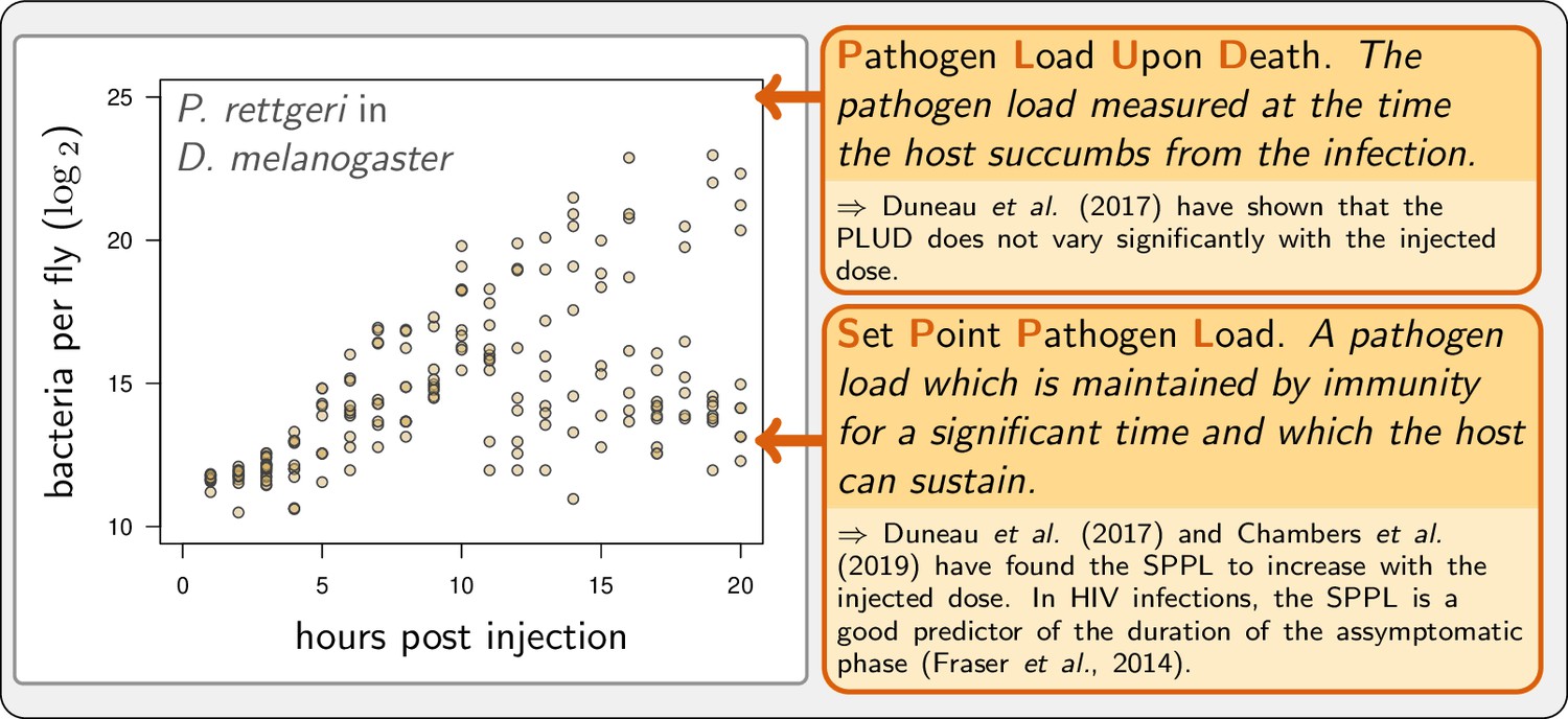
Example of experimental within-host bacterial dynamic using *Drosophila*.

Adapted from Duneau et al., 2017a. Each point represents the bacterial load estimated from a single killed male fly (*Drosophila melanogaster*) injected with a suspension of the bacterium *Providencia rettgeri* containing ca. 2000 bacterial cells. Twenty hours after injection, some flies maintain a moderate load and will live on for several days, while others have reached high loads and will die rapidly.

Figure 2

Download asset Open asset

A model of Within Host Dynamics (WHD).

(A) A description of the model. Large arrows indicate fluxes which make pathogen load ( $x$ ), level of defense ( $y$ ), and damage ( $z$ ) vary over time. Dashed arrows indicate how each variable influences, negatively (flat arrowhead) or positively, these fluxes. Tables list parameters and their default values, separating those which determine the production or efficacy of defense (resistance parameters) from those which determine the production and the repair of damage (tolerance parameters). (B). The activation of defense as described by the functional response $F (x)$ gives the level of defense production that is reached in the absence of negative regulation. It increases with pathogen load $x$ , $F (0) = γ$ (the horizontal gray line) being the maximum constitutive defense production, reached when the host is not infected. $α$ controls how fast defense expression increases with load (dashed curve: $α = 24$ instead of 12 for the plain curve). Increasing $u$ , (dotted curve: $u = 0.75$ instead of 0.5) makes $F$ increase slower when the pathogen load is low. (C) The negative regulation of defense production as described by the functional response $G (y, z)$ . Down-regulation of defense production increases with both defense ( $y$ ) and damage ( $z$ ) levels. Note, however, that $ψ = 0$ or $l = 0$ would make $G$ independent of damage level.

Figure 3

Download asset Open asset

Illustrative cases of infection dynamics.

Each column corresponds to one of the three variables of the model ( $x$ , pathogen load; $y$ , defense; $z$ , damage). In all cases, the initial pathogen load ( $x_{0}$ ) is 10⁻⁶ and, unless otherwise specified, $y_{0}$ and $z_{0}$ are set at their homeostatic state ${\tilde{y}}_{h}$ and ${\tilde{z}}_{h}$ (indicated by horizontal dashed line). Red letters in circles indicate the outcome of the infection: C, clearance; L, low pathogen load; H, high pathogen load. Dots correspond to results of stochastic simulations where the initial pathogen load is randomly drawn from a log-normal distribution with an average in $\log (x_{0})$ set to $\log (10^{- 6})$ and variance 0.15, and then the deterministic equations of the model are solved numerically. (**A-C**) illustrate cases where the immune defense eventually controls the infection, either by clearing pathogens (gray curves, $γ = 5$ ) or by making it chronic (green curves, $γ = 1.8$ ). With $γ = 5$ , the constitutive expression of defense is strong and hence the level of defense before infection ( ${\tilde{y}}_{h}$ ) is very high. This level slightly increases upon infection (which leads to a corresponding increase in damage, as defense induce damage when $η > 0$ ) and returns to the homeostatic state once pathogens have been cleared. With $γ = 1.8$ (green curve), the initial level of defense is much lower and the infection stabilizes at the Set Point Pathogen Load (SPPL, see Figure 1). Defense and damage both peak following infection and, because pathogen are not cleared, they eventually stabilize at a level above the homeostatic state. (**D-F**) illustrates cases where the immune response does not suffice to control the infection (green curves, $γ = 1.8$ , red curves, $γ = 0.5$ ). In both cases, the peak in defense production induced by infection is not sufficient to stop pathogen proliferation. This, combined to the side effects of defense, provokes a sharp increase in damage. The accumulation of damage hinders defense production (because $ψ > 0$ and $l > 0$ ) which in turn makes the level of defense rapidly decrease. The infection is then out of control and eventually kills the host, when the accumulated damage $z$ exceeds the level the host can sustain ( $z > z_{d}$ ). Note that the two hosts die at very similar Pathogen Load Upon Death (PLUD, see Figure 1) although at very different times. Note also that bacteria continue proliferating after host death, so that the PLUD is below the carrying capacity at the time of death (which is fixed to one) and likely much below the load that could be reached in a cadaver. When $γ = 1.8$ (green curve), the immune response is strong enough to curb pathogen proliferation. This maintains the population of pathogens at a SPPL, which differs from that of the green curve in figures **A-C** because it is transient. These two green curves have been obtained with identical parameters; they only differ in the initial level of damage $z_{0}$ (which,in D-F, is increased by 0.3% of $z_{d}$ ). Their differences, therefore, demonstrate that the model can be bistable: with fixed parameters, the outcome of an infection might depend on initial conditions. These simulations can be reproduced using a dedicated R Shiny web application (Chang et al., 2021), where parameter values can be changed to explore their impact on the dynamics (see https://plafont.shinyapps.io/WHD_app/, DOI: 10.5281/zenodo.13309653).

Figure 4

Download asset Open asset

Constitutive and inducible defense production determine bistability and infection outcome.

(A) The types of stable equilibria when maximum rate of constitutive defense production (γ) and defense activation rate (α) vary. Parameters are as in Figure 2 and both α and γ are varied. The vertical dashed line indicates the value of $γ_{c}$ above which clearance is stable. Red labels indicate which equilibria are stable: H, high load equilibrium, L, low load equilibrium and C, clearance (the distinction between H and L equilibrium is exemplified in figures **B and C**). The two oblique solid lines delimit a parameter region for which the system is bistable (H/L or H/C). The color indicates which equilibrium the infection actually reaches when the initial load is $x_{0} = 10^{- 6}$ and when $y_{0}$ and $z_{0}$ are set to the homeostatic state. (B) The equilibrium load $\tilde{x}$ as a function of α when parameters are as in A but γ is fixed to 2 (which corresponds to the vertical dotted line in A). Solid lines indicate stable equilibria while dashed lines are unstable ones. The distinction between high load and low-load equilibria is appropriate here because equilibria with intermediate loads are not stable. (C) The equilibrium load $\tilde{x}$ as a function of γ with parameters as in A except α fixed to 10 (which corresponds to the horizontal dotted line in A). In the bistable region, the high load equilibrium is always possible; the second possible equilibrium is either low load, when γ is below $γ_{c}$ , or clearance otherwise. (D) Parameters as in A except $ψ = 0.5$ , which reduces the negative impact of damage on defense production. (E) Parameters as in A except $u = 0.75$ , which lowers defense production at low pathogen load.

Figure 5

Download asset Open asset

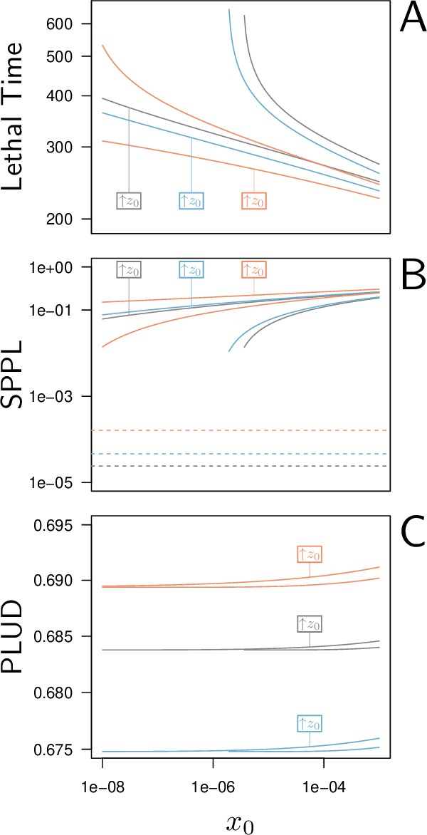
Lethal Time, Set-Point Pathogen Load (SPPL), and Pathogen Load Upon Death (PLUD) are three measurable quantities which reflect both resistance and tolerance.

The three quantities are represented here as functions of the inoculated dose. The black curves have been computed with parameters as in Figure 2, while the red curves correspond to a decrease in resistance (5% decrease in defense efficiency $δ$ ) and the blue to a decrease in tolerance (5% decrease in damage repair efficiency $ξ$ ). For each parameter set, $y_{0}$ was set at its homeostatic state and $z_{0}$ was either at the homeostatic state or increased by 1% of $z_{d}$ (indicated by boxes in the figures). (A) The Lethal Time (LT) decreases with inoculated dose and with $z_{0}$ . Decrease in resistance or in tolerance both reduces the time it takes for the pathogen to kill the host. Note that a decrease in tolerance (blue curves compared to black curves) only shifts the relationship between LT and dose, without altering its slope. (B) The stable SPPL (dashed lines) is by definition independent from initial conditions. The transient SPPL (solid lines) conversely increases with both $x_{0}$ and $z_{0}$ . Decreased resistance and decreased tolerance both increase the SPPL. Variations in transient SPPL mirror that of LT, which indicates that the SPPL is a good predictor of the host lifespan. (C) The PLUD is almost independent from the initial dose and slightly increases with $z_{0}$ . It increases with lowered resistance (low $δ$ , red curves) but decreases when tolerance is lowered (low $ξ$ , blue curves).

Figure 6

Download asset Open asset

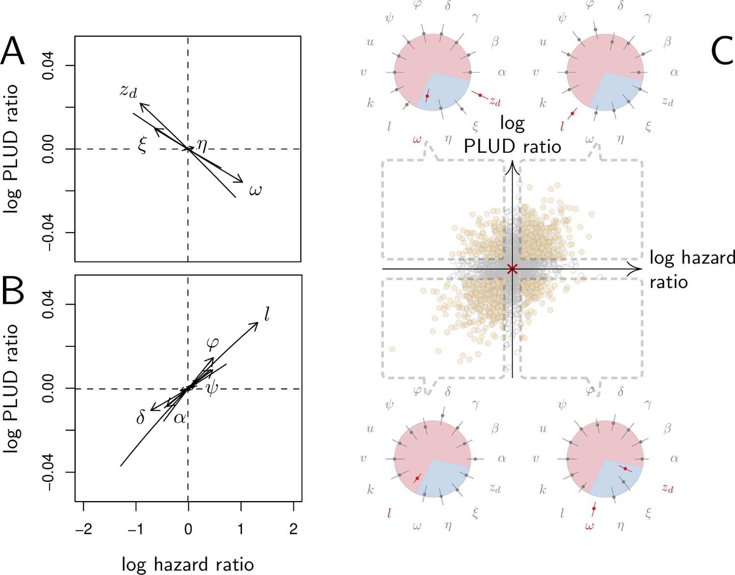
Effect of parameter variations on Pathogen Load Upon Death (PLUD) and hazard ratio (HR).

In (**A and B**), parameters are initially fixed as in Figure 2 except for $γ = 0.5$ , as in red curve if Figure 3. Parameters are then varied one at a time, from –5 to +5%. For each modified parameter value, the PLUD was computed and 100 survival simulations were run with $x_{0}$ randomly drawn from a log-normal distribution with average 10⁻⁶ and variance 0.5. A Cox proportional hazard model was then fitted on simulated data so that log Hazard Ratio (log HR) could be related to parameter variation. The horizontal dashed lines would correspond to parameters which have no influence on PLUD; the vertical dashed line would correspond to those which do not impact HR. (A) The effect of tolerance parameters (defined as in Figure 2A). Arrows indicate that, as expected, any increase in the damage induced by the pathogen ( $ω$ ) decrease the PLUD, while increasing damage repair ( $ξ$ ) or tolerance to damage ( $z_{d}$ ) has the opposite effects. For the parameter set we have used here, increasing $η$ has almost no effect on PLUD and only slightly increases HR. (B) The effects of resistance parameter (defined as in Figure 2A). Variation in any of these parameters produces a positive correlation between PLUD and HR. (C) The variation in PLUD and HR when all parameters are all randomly drawn from independent Gaussian laws. The red cross corresponds to a strain with parameters as in Figure 2 and each dot is a ‘mutant strain’ which parameters have 95% chances to deviate by less than 0.5% from that of the ‘wild-type strain.’ Open circles are mutants which either log PLUD ratio or log HR ratio do not significantly deviate from zero (see text for details). We sorted mutants in four groups, according to whether their PLUD and HR has significantly increased or decreased compared to the wild strain. The distributions of traits are indicated for each group on colored circles, with segments spanning 75% of the deviation range and the central dot corresponding to the median deviation. Segments in red indicate that 75% of the mutants have either lower trait values than the wild-type strain (when the segment is inside the circle) or higher trait values (when outside).

Figure 7

Download asset Open asset

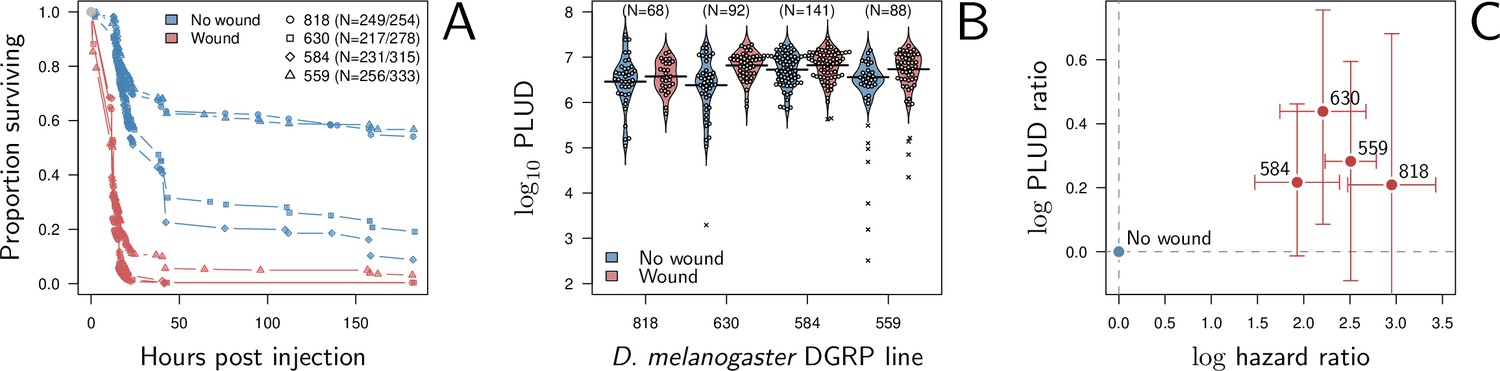
Hazard ratio (HR) and Pathogen Load Upon Death (PLUD) estimations on D. *melanogaster* infected with *Providencia rettgeri* with or without thorax wound prior to injection.

We performed the experiment on four genotypes sampled from the *Drosophila* Genetic Reference Panel (lines RAL-818, RAL-630, RAL-584 and RAL-559, which have no known difference in immunity effectors). (A) Proportion of surviving flies as a function of hours post injection. Numbers in legend indicate sample sizes for no wound/wound treatments, respectively. In all lines, the wound significantly and sharply reduces survival. (B) PLUD for each *D. melanogaster* line. Each point represents an individual fly and the bars represent the means. Crosses are PLUD estimates which have been categorized as outliers by a Rosner test. (C) Log PLUD ratio as a function of log Hazard Ratio. For each line, we computed the log-ratio of PLUD in wounded flies to that in non-wounded (with outliers excluded). The value of zero, therefore, corresponds to a non-wounded reference, as for log-HR. Bars represents the 95% CI obtained by bootstrap. The wound consistently increases both the HR and the PLUD, as our model predicts.

Figure 8

Download asset Open asset

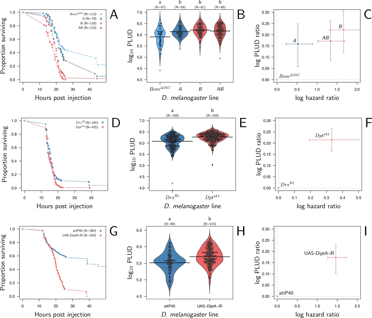
Hazard ratio (HR) and Pathogen Load Upon Death (PLUD) estimations in immuno-deficient lines of D. *melanogaster* infected with *Providencia rettgeri*.

(A, D, and G) give the proportion of surviving flies as a function of hours post-injection. (B, E, and H) present per fly estimations of PLUD. Black lines represent the means, different symbols correspond to distinct replicate experiments, and small letters above graph indicate significant differences, as tested by a pairwise Wilcoxon test. (**C, F, and I**) present per line estimations of log PLUD ratios, as a function of estimations of log HR. Ratios are here computed relative to the control line and bars represents the 95% CI as obtained by bootstrap. In (**A-C**), three lines which lack effectors active against *P. rettgeri* (A Defensin deleted, B all Diptericins deleted and AB both Defensin and Diptericins deleted) are compared to *Bom*^Δ55C. *Bom*^Δ55C lacks Bomanins, immune effectors which are inactive against *P. rettgeri*, and is thus used here as a control. All three lines die significantly faster than *Bom*^Δ55C and have a significantly higher PLUD (**B and C**). In panels (**D-F**), following a similar logic, we compared *DptA*^SK1, which has Diptericin A deleted, to *Drs*^R1, which has Drosomycin deleted. Diptericin A has been shown to be the most active AMP against *P. rettgeri* while Drosomycin is active mostly against gram positive bacteria and fungi. (D) demonstrates that deleting Diptericin A is sufficient to make the mutant more susceptible to the infection than *Drs* mutant. (E and F) demonstrate that this increase in susceptibility goes together with an increase in PLUD. In (G-I) we used RNAi to silence Diptericin A. The control is the match genetic background recommended for the TRiP RNAi panel. Silencing Diptericin A accelerates death (G) and significantly increases the PLUD (**H-I**).

Figure 9

Download asset Open asset

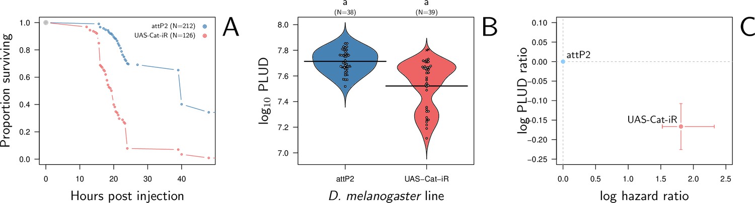
Hazard ratio (HR) and Pathogen Load Upon Death (PLUD) estimations in D. *melanogaster* with RNAi-silenced Catalase infected with *Providencia rettgeri*.

As in Figure 8G–I, the control is the match genetic background recommended for the TRiP RNAi panel. Silencing Catalase accelerates death (panel A) and significantly decreases the PLUD (panels **B-C**).

Appendix 1—figure 1

Download asset Open asset

The dynamics of the system in a bistable configuration.

Appendix 2—figure 1

Download asset Open asset

Elasticity analysis of equilibrium load.

Parameters are here as in Figure 2 and the derivatives of log equilibrium load $\tilde{x}$ relative to log parameters, obtained from , are computed for the low load equilibrium. For this equilibrium, $\tilde{x}$ is the load at which the chronic infection stabilizes and can, therefore, be considered as a stable Set-Point Pathogen Load (SPPL). The parameters with greatest influence on SPPL are first the efficiency of defense ( $δ$ ) and second the parameter which shapes the impact of damage on defense production ( $l$ ).

Appendix 3—figure 1

Download asset Open asset

The influence of initial conditions on transient Set-Point Pathogen Load (SPPL).

Left panel: each graph represents the partial derivative of log-SPPL relative to log-transformed inoculum size ( $\log (x_{0})$ , first column), pre-infection level of defense ( $\log (y_{0})$ , second column) and pre-infection level of damage ( $\log (z_{0})$ , third column) with $x_{0} = 10^{- 6}$ and $y_{0}$ and $z_{0}$ set to the homeostatic state. In the first row, parameters are set as in Figure 2, while $ψ = 0.5$ in the second row, and $ξ = 0.015$ in the third. The vertical dashed line is the value $γ_{c}$ of γ, above which clearance is stable. Two black curves (with only one visible except when $ψ = 0.5$ ) delimits the parameter region in which the system is bistable. Within this region, the solid and dashed dark-red curves delimit a sub-region where the SPPL is transient in the conditions of the simulations. Below the red curve (which is visible only when $ψ = 0.5$ or $ξ = 0.015$ ) a high load infection always kills the host. The case $u = 0.75$ , which we analyzed in Figure 4, is not presented here as the SPPL cannot be transient in this condition. The blue color indicates better control of the infection, i.e., decreased SPPL, while red means increased SPPL. In each case, anything that weakens the host (higher $x_{0}$ , lower $y_{0}$ or higher $z_{0}$ ) lowers the SPPL. The analysis also indicates that sensitivity to variations in $y_{0}$ and $z_{0}$ increase with both α and γ. Right panel: This analysis follows the same logic but the partial derivatives of the log of the duration of chronicity are computed. The blue color indicates again better control, i.e., longer chronicity. In most cases, anything that weakens the host shortens control. But conditions exist where this is not true (e.g. in second and third rows when γ and α are low). Contrary to what is expected, chronicity may, therefore, last longer with increased SPPL when immunity is weak.

Appendix 3—figure 2

Download asset Open asset

Elasticity analysis of Set-Point Pathogen Load (SPPL) in transient chronicity according to parameters.

Each graph represents the partial derivative of log SPPL with respect to one (log-transformed) parameter, as a function of α and γ. Blue color corresponds to negative derivatives (i.e. increasing the parameter lowers the SPPL) while red indicates positive derivatives (i.e. increasing the parameter increases the SPPL). The pairs of rows correspond to the three parameter sets studied in Appendix 3—figure 1. Derivatives with respect to $z_{d}$ have been omitted in this analysis as, by definition, $z_{d}$ has no influence on SPPL. The vertical dashed line is the value $γ_{c}$ of γ, above which clearance is stable. Two black curves (with only one visible except when $ψ = 0.5$ ) delimits the parameter region in which the system is bistable. Within this region, the solid and dashed dark-red curves delimit a sub-region where the SPPL is transient in the conditions of the simulations. Below the red curve (which is visible only when $ψ = 0.5$ or $ξ = 0.015$ ) a high load infection always kills the host.

Appendix 3—figure 3

Download asset Open asset

Elasticity analysis of the duration of transient chronicity according to parameters.

Each graph represents the partial derivative of the log duration of chronicity with respect to one (log-transformed) parameter, as a function of α and γ. Blue color corresponds to positive derivatives (i.e. increasing the parameter lengthen chronicity) while red indicates negative derivatives (i.e. increasing the parameter shortens chronicity). The three pairs of rows correspond to the three parameter sets studied in Appendix 3—figure 1. Derivatives with respect to $z_{d}$ have been omitted in this analysis as, by definition, $z_{d}$ has no influence on Set-Point Pathogen Load (SPPL). The vertical dashed line is the value $γ_{c}$ of γ, above which clearance is stable. Two black curves (with only one visible except when $ψ = 0.5$ ) delimits the parameter region in which the system is bistable. Within this region, the solid and dashed dark-red curves delimit a sub-region where the SPPL is transient in the conditions of the simulations. Below the red curve (which is visible only when $ψ = 0.5$ or $ξ = 0.015$ ) a high load infection always kills the host.

Appendix 4—figure 1

Download asset Open asset

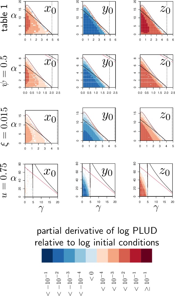
Elasticity analysis of the Pathogen Load Upon Death (PLUD) relative to initial conditions.

Each graph represents the partial derivative of log-PLUD relative to log-transformed inoculum size ( $\log (x_{0})$ , first column), pre-infection level of defense ( $\log (y_{0})$ , second column) and pre-infection level of damage ( $\log (z_{0})$ , third column) with $x_{0} = 10^{- 6}$ and $y_{0}$ and $z_{0}$ set to the homeostatic state. In the first row, parameters are set as in Figure 2, while $ψ = 0.5$ in the second row, $ξ = 0.015$ in the third and $u = 0.75$ in the fourth. The blue color indicates that the PLUD decreases, while red means that PLUD increases. In each case, anything that weakens the host (higher $x_{0}$ , lower $y_{0}$ or higher $z_{0}$ ) increases the PLUD although the effect of dose ( $x_{0}$ ) is really weak. In the particular case $u = 0.75$ , the dependence on $x_{0}$ is so low that numerical derivatives of PLUD cannot be distinguished from zero. The vertical dashed line is the value $γ_{c}$ of $γ$ , above which clearance is stable. Two black curves (with only one visible except when $ψ = 0.5$ or $u = 0.75$ ) delimits the parameter region in which the system is bistable. Within this region, the solid and dashed dark-red curves delimit a sub-region where the Set-Point Pathogen Load (SPPL) is transient in the conditions of the simulations (except when $u = 0.75$ , where this never happens). Below the red curve (which is visible only when $ψ = 0.5$ or $u = 0.75$ ) a high load infection always kills the host.

Appendix 4—figure 2

Download asset Open asset

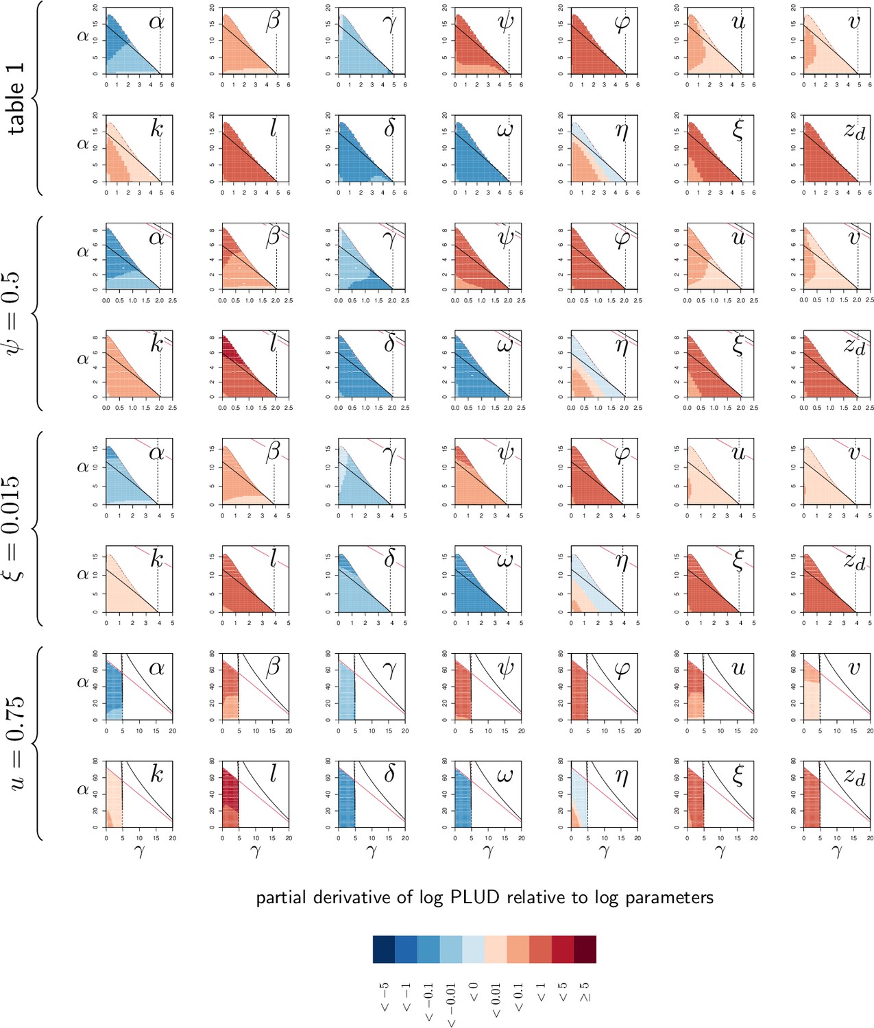
Elasticity analysis of Pathogen Load Upon Death (PLUD).

Each graph represents the partial derivative of PLUD with respect to one parameter, as a function of α and γ. Blue color corresponds to negative derivatives (i.e. increasing the parameter decreases the PLUD) while red indicate positive derivatives (i.e. increasing the parameter increases the PLUD). The black curves delimit the region of bistability, as in Figure 4; above the red line, the equilibrium $z$ is below $z_{d}$ even for the most severe infection. The four braces correspond to the four parameter sets studied in Figure 4. The vertical dashed line indicates $γ_{c}$ . Black and red curves are as in Appendix 4—figure 1.

Appendix 5—figure 1

Download asset Open asset

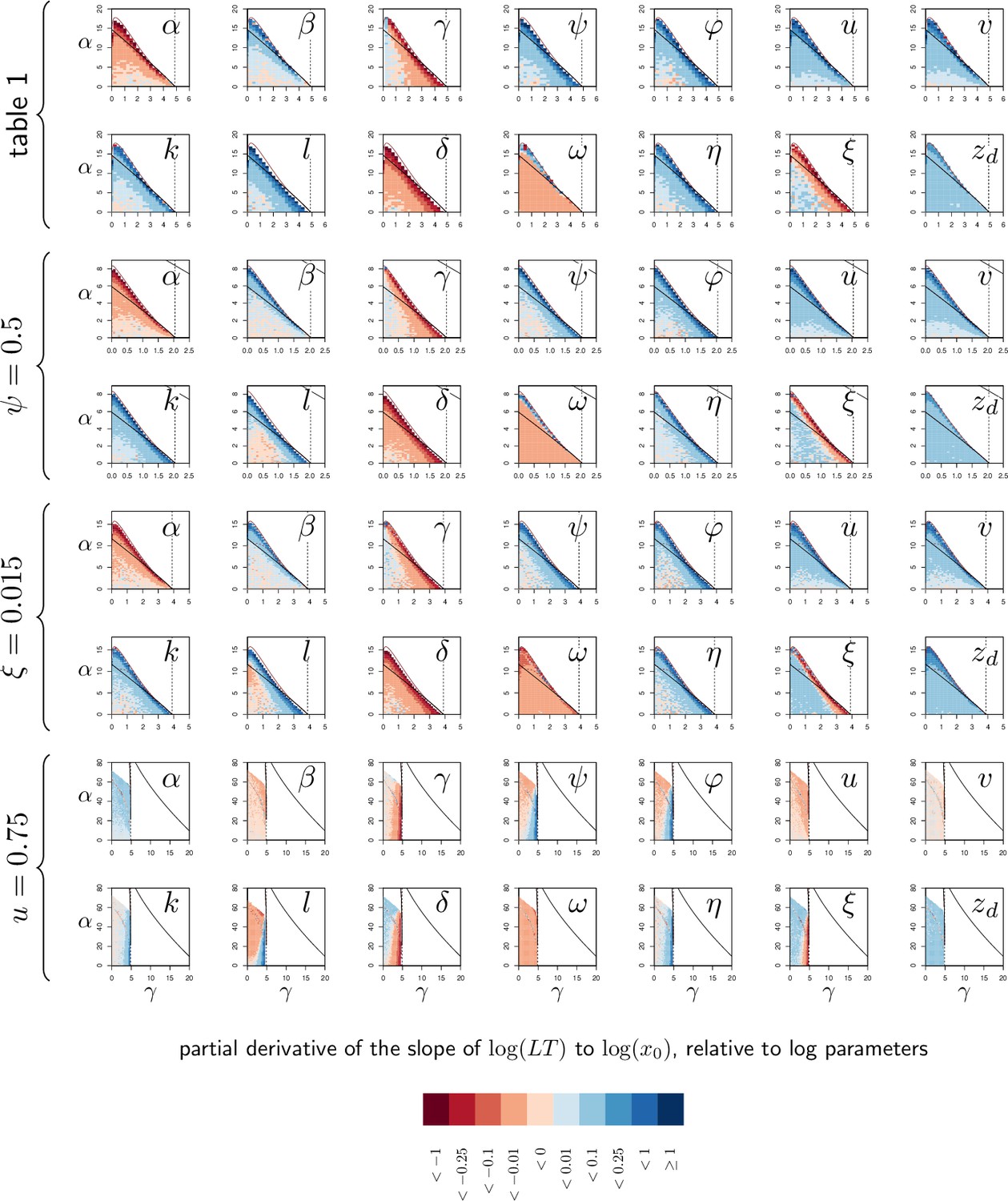
Elasticity analysis of the Slope of Lethal Time (LT) to dose.

Each graph represents the partial derivative of hazard ratio with respect to one parameter, as a function of $α$ and $γ$ . Blue color corresponds to positive derivatives (i.e. increasing the variable brings the slope closer to zero) while red indicate negative derivatives. The black curves delimit the region of bistability, as in Figure 4; above the red line, the equilibrium $\tilde{z}$ never exceeds $z_{d}$ so that the infection cannot kill the host. Each of the four rows corresponds to one of the parameter sets studied in Figure 4. The vertical dashed line indicates $γ_{c}$ . Black and red curves are as in Appendix 4—figure 1.

Appendix 6—figure 1

Download asset Open asset

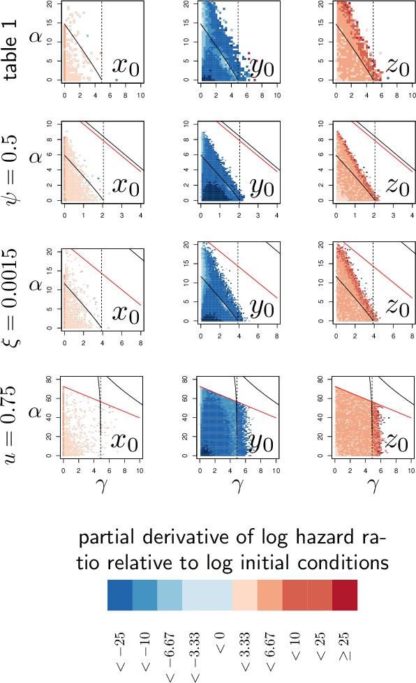
Elasticity analysis of Hazard Ratio, relative to initial conditions.

Each graph represents the partial derivative of log(HR) with respect to the log-transformed initial state of one variable, as a function of α and γ. Blue color corresponds to negative derivatives (i.e. increasing the variable decreases hazard ratio, HR) while red indicate positive derivatives. The black curves delimit the region of bistability, as in Figure 4; above the red line, the equilibrium $\tilde{z}$ never exceeds $z_{d}$ so that the infection cannot kill the host. Each of the four row corresponds to one of the parameter sets studied in Figure 4. The vertical dashed line indicates $γ_{c}$ . Black and red curves are as in Appendix 4—figure 1.

Appendix 6—figure 2

Download asset Open asset

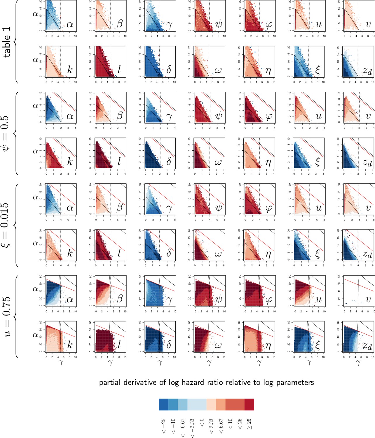
Elasticity analysis of Hazard Ratio, relative to parameters.

Each graph represents the partial derivative of hazard ratio with respect to one parameter, as a function of $α$ and $γ$ . Blue color corresponds to negative derivatives (i.e. increasing the variable decreases HR) while red indicate positive derivatives. The black curves delimit the region of bistability, as in Figure 4; above the red line, the equilibrium $\tilde{z}$ never exceeds $z_{d}$ so that the infection cannot kill the host. Each of the four rows corresponds to one of the parameter sets studied in Figure 4. The vertical dashed line indicates $γ_{c}$ . Black and red curves are as in Appendix 4—figure 1.

Appendix 7—figure 1

Download asset Open asset

The distribution of log Pathogen Load Upon Death (PLUD) as a function of the proportion of individuals which did not die from the infection in a chosen simulated sample of 50 individuals.

Background mortality was assumed to be constant so that death time in the absence of infection are exponentially distributed. An individual was considered as killed by the infection if the time to death predicted by our model was lower than the time randomly drawn in an exponential distribution. The average of the exponential distribution was adjusted sa that we could control the proportion of individuals which did not die from the infection (represented by large dots). Red dots indicate outliers as detected by a Rosner test. PLUD was simulated with $δ = 0.125$ , $φ = 0.015$ , $γ = 3$ , $α = 10$ , $β = 1$ , $u = 0.1$ , $v = 0.1$ , $k = 0.5$ , $ψ = 2$ , $l = 1.5$ , $ω = 10$ , $η = 0.01$ , $ξ = 0.01$ , $z_{d} = 100$ so that the simulated distribution mimics that of experimental results.

Appendix 7—figure 1—source data 1 Protocol of dilution to estimate the Pathogen Load Upon Death (PLUD).: https://cdn.elifesciences.org/articles/104052/elife-104052-app7-fig1-data1-v2.xlsx
Download elife-104052-app7-fig1-data1-v2.xlsx

Appendix 7—figure 2

Download asset Open asset

Proportion of detected outliers using a Rosner test, with background mortality producing exponentially distributed death times (i.e. Weibull distribution with shape parameter equals one).

The proportion of Pathogen Load Upon Death (PLUD) values detected as outliers adequately reflects the proportion of individuals which died from causes other than infection. We simulated here 100 samples of 50 individual PLUD values and ran a Rosner test on each sample, using a five percent threshold p-value.

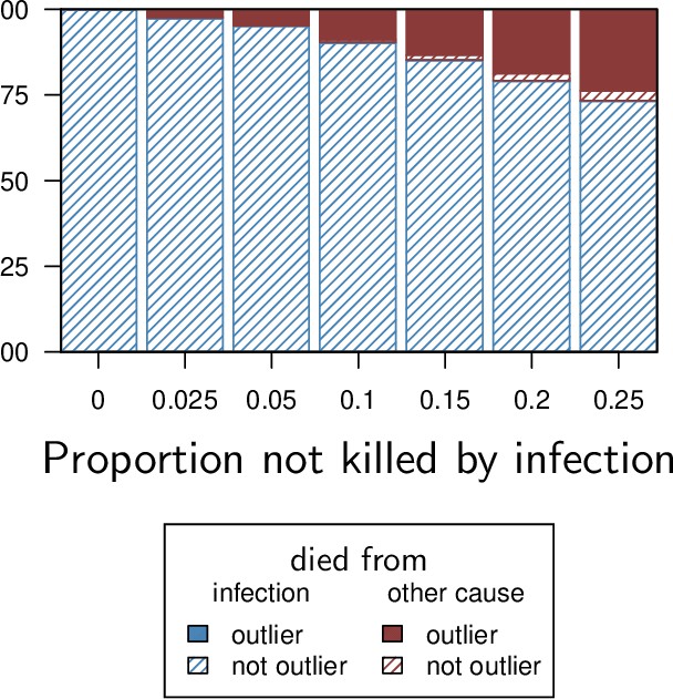
Appendix 7—figure 3

Download asset Open asset

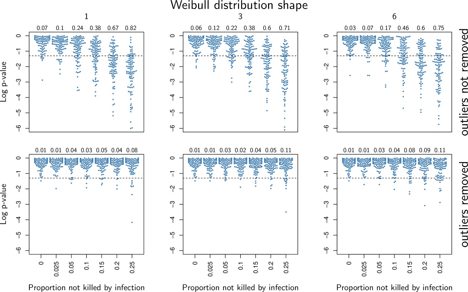
p-values of a Wilcoxon rank test where two 50 individuals samples were compared, one where all individuals died from the infection and another where some individuals died from other causes.

Each column corresponds to a different shape of Weibull distribution, 1 being the case where natural death rate is constant over time, 3 and 6 being being cases where natural death rate increases with age. Numbers given in the top margin of the graphs indicate the proportion of tests (out of 100) which yielded a significant difference, using a 0.05 significance level. In the first row, the presence of individuals which did not die from the infection creates significant Pathogen Load Upon Death (PLUD) difference. In the second row, a Rosner test is applied to detect outliers before the Wilcoxon test is run. The proportion of test yielding significant difference is markedly reduced in this situation.

Tables

Appendix 2—table 1

Derivatives of equilibrium load with respect to model parameters. For each parameter, the derivative is given together with its sign for stable and unstable equilibria.

	$\partial \tilde{x} / \partial \cdot$	st. eq.	unst. eq.
$δ$	$\begin{aligned} - \frac{φ \tilde{y}}{δ} (k {\tilde{y}}^{k} + \frac{ψ η}{ξ} l \tilde{y} {\tilde{z}}^{l - 1}) \times \frac{G (\tilde{y}, \tilde{z})}{H^{'} (\tilde{x})} \\ - \frac{φ}{δ} \tilde{y} \times \frac{1}{H^{'} (\tilde{x})} \end{aligned}$	$< 0$	$> 0$
$α$	$- \frac{{\tilde{x}}^{u}}{1 + β {\tilde{x}}^{v}} \times \frac{G (\tilde{y}, \tilde{z})}{H^{'} (\tilde{x})}$	$< 0$	$> 0$
$β$	$α \frac{{\tilde{x}}^{u}}{1 + β {\tilde{x}}^{v}} \times \frac{G (\tilde{y}, \tilde{z})}{H^{'} (\tilde{x})}$	$> 0$	$< 0$
$γ$	$- \frac{G (\tilde{y}, \tilde{z})}{H^{'} (\tilde{x})}$	$< 0$	$> 0$
$ψ$	$φ \tilde{y} {\tilde{z}}^{l} \times \frac{G (\tilde{y}, \tilde{z})}{H^{'} (\tilde{x})}$	$> 0$	$< 0$
$φ$	$\tilde{y} \times \frac{1}{H^{'} (\tilde{x})}$	$> 0$	$< 0$
$u$	$- l o g (\tilde{x}) (F (\tilde{x} - γ)) \times \frac{G (\tilde{y}, \tilde{z})}{H^{'} (\tilde{x})}$	$> 0$	$< 0$
$v$	$l o g (\tilde{x}) \frac{α β {\tilde{x}}^{u + v}}{(1 + β \tilde{x})^{2}} \times \frac{G (\tilde{y}, \tilde{z})}{H^{'} (\tilde{x})}$	$< 0$	$> 0$
$k$		$> 0 i f \tilde{y} > 1$	$< 0 i f \tilde{y} > 1$
	$l o g (\tilde{y}) ψ φ {\tilde{y}}^{k + 1} \times \frac{G \tilde{y}, \tilde{z}}{H^{'} (\tilde{x})}$	$> 0 i f \tilde{z} > 1$	$< 0 i f \tilde{z} > 1$
	$\frac{φ ψ l}{ξ} \tilde{x} \tilde{y} {\tilde{z}}^{l - 1} \times \frac{G \tilde{y}, \tilde{z}}{H^{'} (\tilde{x})}$	$> 0$	$< 0$
$η$	$\frac{φ ψ l}{ξ} {\tilde{y}}^{2} {\tilde{z}}^{l - 1} \times \frac{G \tilde{y}, \tilde{z}}{H^{'} (\tilde{x})}$	$> 0$	$< 0$
$ξ$	$- \frac{φ ψ l}{ξ} \tilde{y} {\tilde{z}}^{l} \times \frac{G \tilde{y}, \tilde{z}}{H^{'} (\tilde{x})}$	$< 0$	$> 0$

Additional files

MDAR checklist: https://cdn.elifesciences.org/articles/104052/elife-104052-mdarchecklist1-v2.docx
Download elife-104052-mdarchecklist1-v2.docx
Source code 1 Rmarkdown file including codes and analyses associated with the experimental data.: https://cdn.elifesciences.org/articles/104052/elife-104052-code1-v2.zip
Download elife-104052-code1-v2.zip
Appendix 7—figure 1—source data 1 Protocol of dilution to estimate the Pathogen Load Upon Death (PLUD).: https://cdn.elifesciences.org/articles/104052/elife-104052-app7-fig1-data1-v2.xlsx
Download elife-104052-app7-fig1-data1-v2.xlsx

Download links

A two-part list of links to download the article, or parts of the article, in various formats.

Downloads (link to download the article as PDF)

Article PDF

Open citations (links to open the citations from this article in various online reference manager services)

Mendeley

Cite this article (links to download the citations from this article in formats compatible with various reference manager tools)

David Duneau
Pierre DM Lafont
Christine Lauzeral
Nathalie Parthuisot
Christian Faucher
Xuerong Jin
Nicolas Buchon
Jean-Baptiste Ferdy

(2025)

A within-host infection model to explore tolerance and resistance

eLife 14:e104052.

https://doi.org/10.7554/eLife.104052

Figures

Example of experimental within-host bacterial dynamic using Drosophila.

A model of Within Host Dynamics (WHD).

Illustrative cases of infection dynamics.

Constitutive and inducible defense production determine bistability and infection outcome.

Lethal Time, Set-Point Pathogen Load (SPPL), and Pathogen Load Upon Death (PLUD) are three measurable quantities which reflect both resistance and tolerance.

Effect of parameter variations on Pathogen Load Upon Death (PLUD) and hazard ratio (HR).

Hazard ratio (HR) and Pathogen Load Upon Death (PLUD) estimations on D. melanogaster infected with Providencia rettgeri with or without thorax wound prior to injection.

Hazard ratio (HR) and Pathogen Load Upon Death (PLUD) estimations in immuno-deficient lines of D. melanogaster infected with Providencia rettgeri.

Hazard ratio (HR) and Pathogen Load Upon Death (PLUD) estimations in D. melanogaster with RNAi-silenced Catalase infected with Providencia rettgeri.

The dynamics of the system in a bistable configuration.

Elasticity analysis of equilibrium load.

The influence of initial conditions on transient Set-Point Pathogen Load (SPPL).

Elasticity analysis of Set-Point Pathogen Load (SPPL) in transient chronicity according to parameters.

Elasticity analysis of the duration of transient chronicity according to parameters.

Elasticity analysis of the Pathogen Load Upon Death (PLUD) relative to initial conditions.

Elasticity analysis of Pathogen Load Upon Death (PLUD).

Elasticity analysis of the Slope of Lethal Time (LT) to dose.

Elasticity analysis of Hazard Ratio, relative to initial conditions.

Elasticity analysis of Hazard Ratio, relative to parameters.

The distribution of log Pathogen Load Upon Death (PLUD) as a function of the proportion of individuals which did not die from the infection in a chosen simulated sample of 50 individuals.

Appendix 7—figure 1—source data 1

Proportion of detected outliers using a Rosner test, with background mortality producing exponentially distributed death times (i.e. Weibull distribution with shape parameter equals one).

p-values of a Wilcoxon rank test where two 50 individuals samples were compared, one where all individuals died from the infection and another where some individuals died from other causes.

Tables

Derivatives of equilibrium load with respect to model parameters. For each parameter, the derivative is given together with its sign for stable and unstable equilibria.

Additional files

MDAR checklist

Source code 1

Appendix 7—figure 1—source data 1

Download links

Downloads (link to download the article as PDF)

Open citations (links to open the citations from this article in various online reference manager services)

Cite this article (links to download the citations from this article in formats compatible with various reference manager tools)

Be the first to read new articles from eLife

Share this article

Cite this article

Example of experimental within-host bacterial dynamic using Drosophila.

A model of Within Host Dynamics (WHD).

Illustrative cases of infection dynamics.

Constitutive and inducible defense production determine bistability and infection outcome.

Lethal Time, Set-Point Pathogen Load (SPPL), and Pathogen Load Upon Death (PLUD) are three measurable quantities which reflect both resistance and tolerance.

Effect of parameter variations on Pathogen Load Upon Death (PLUD) and hazard ratio (HR).

Hazard ratio (HR) and Pathogen Load Upon Death (PLUD) estimations on D. melanogaster infected with Providencia rettgeri with or without thorax wound prior to injection.

Hazard ratio (HR) and Pathogen Load Upon Death (PLUD) estimations in immuno-deficient lines of D. melanogaster infected with Providencia rettgeri.

Hazard ratio (HR) and Pathogen Load Upon Death (PLUD) estimations in D. melanogaster with RNAi-silenced Catalase infected with Providencia rettgeri.

The dynamics of the system in a bistable configuration.

Elasticity analysis of equilibrium load.

The influence of initial conditions on transient Set-Point Pathogen Load (SPPL).

Elasticity analysis of Set-Point Pathogen Load (SPPL) in transient chronicity according to parameters.

Elasticity analysis of the duration of transient chronicity according to parameters.

Elasticity analysis of the Pathogen Load Upon Death (PLUD) relative to initial conditions.

Elasticity analysis of Pathogen Load Upon Death (PLUD).

Elasticity analysis of the Slope of Lethal Time (LT) to dose.

Elasticity analysis of Hazard Ratio, relative to initial conditions.

Elasticity analysis of Hazard Ratio, relative to parameters.

The distribution of log Pathogen Load Upon Death (PLUD) as a function of the proportion of individuals which did not die from the infection in a chosen simulated sample of 50 individuals.

Appendix 7—figure 1—source data 1

Proportion of detected outliers using a Rosner test, with background mortality producing exponentially distributed death times (i.e. Weibull distribution with shape parameter equals one).

p-values of a Wilcoxon rank test where two 50 individuals samples were compared, one where all individuals died from the infection and another where some individuals died from other causes.

Derivatives of equilibrium load with respect to model parameters. For each parameter, the derivative is given together with its sign for stable and unstable equilibria.

MDAR checklist

Source code 1

Appendix 7—figure 1—source data 1

Downloads (link to download the article as PDF)

Open citations (links to open the citations from this article in various online reference manager services)

Cite this article (links to download the citations from this article in formats compatible with various reference manager tools)