A stochastic explanation for observed local-to-global foraging states in Caenorhabditis elegans
- Department of Biology, Johns Hopkins University, United States
- David Geffen School of Medicine, University of California, United States
- Solomon H. Snyder Department of Neuroscience, Johns Hopkins University, United States
Figures
Figure 1
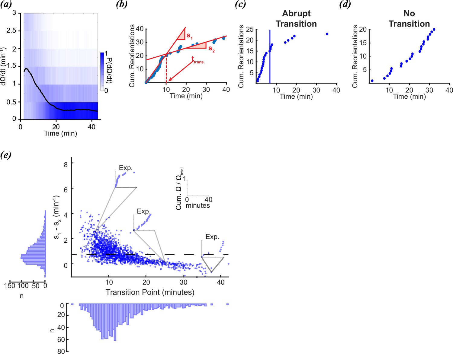
Foraging kinetics of C.elegans.
(a) Average experimental population reorientation rate (black line) in a rolling 2 min window. Blue bins represent probability of observed reorientation rate. (b) Abrupt transitions were identified by performing two linear regressions on observed reorientation curves. Transition times (trans) were defined by the intersection of the regressions (dashed line). The slopes of the two regressions are s1 and s2. (c) An example of an experimental reorientation curve with an abrupt reorientation transition (marked by vertical line). (d) An example of an experimental reorientation curve that lacked an abrupt reorientation transition. (e) Distribution of slope differences and transition times from regressions fit to the experimental data. Individual data points are individual reorientation data for each worm. Insets are individual examples of experimental cumulative reorientation curves. Number of worms (N)=1631. Dashed line represents the median slope difference. All data curated from López-Cruz et al., 2019.
Figure 2
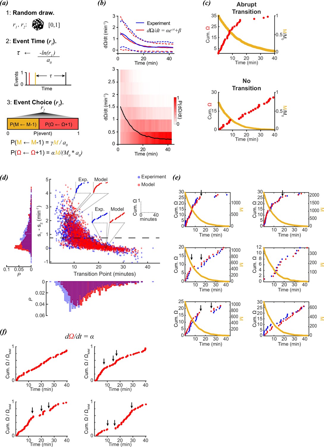
Stochastic modeling of foraging kinetics of C. elegans.
(a) Outline of the Gillespie algorithm. Step 1: Two random numbers (r1 and r2) are drawn from a uniform distribution [0,1]. Step 2: The time interval for a new event (τ) is randomly assigned based on the total propensities (a0) and r1. Step 3: The event i (either a decay of M (M←M-1) or a new reorientation (Ω←Ω+1)) at t + τ is determined by the probability (P(i)) of the event i occurring. This probability is determined by the relative propensity (ai/a0) of the event i. (b) (Top) The parameters α, β, and γ are assigned based on fitting a decay curve (red) to the observed average reorientation rate (blue). Dashed lines are + and – standard deviation. (Bottom) Average model population reorientation rate (black line) in a rolling 2 min window. Red bins represent the probability of observed reorientation rate. N=1631, α=1.49 min–1, β=0.1937 min–1, γ=0.11 min–1. (c) (Top) An example of a modeled abrupt reorientation transition. (Bottom) An example of a modeled reorientation curve that lacked an abrupt reorientation transition. Red data are cumulative reorientations and orange data are M. (d) Distribution of slope differences and transition times from regressions fit to the experimental (blue) and modeled (red) data. Individual data points are individual reorientation data for experimental (blue) or in silico (red) worms. Insets are individual examples of experimental and modeled cumulative reorientation curves. Dashed line represents the median experimental slope difference. (e) Examples of experimental (blue) and modeled (red) cumulative reorientation curves for individual worms, with similar stochastic dynamics. For each example drawn from experiments (blue), the in silico worm with the highest correlation from N=1631 iterations is shown (red). Sudden changes in rate are indicated with arrows. M for each example is shown in orange. (f) Examples of modeled data when the reorientation rate is constant (=1.5). Sudden changes in rate are indicated with arrows.
Figure 3
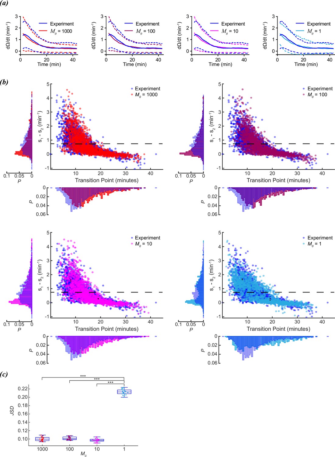
Scaling of foraging kinetics of C. elegans.
(a) Average reorientation rates for experiments (blue), and models where M0=1000 (red), M0=100 (plum), M0=10 (magenta), or M0=1 (cyan). Dashed lines indicate standard deviation. (b) Distribution of slope differences and transition times from regressions fit to the experimental data (blue), and models where M0=1000 (red), M0=100 (plum), M0=10 (magenta), or M0=1 (cyan). Number of worms for both experiment and models (N)=1631. Dashed line represents the median slope difference for the experimental data. (c) The Jensen-Shannon divergence between the experimental distribution for slope difference and transition time in (b), and the distributions generated from models where M0=1,000 (red), M0=100 (plum), M0=10 (magenta), or M0=1 (cyan). Twenty distributions were generated for each M0 model. Quartiles represented by box and whiskers. P-values calculated using Tukey’s range test: <0.001: ***.
Download links
A two-part list of links to download the article, or parts of the article, in various formats.
Downloads (link to download the article as PDF)
Open citations (links to open the citations from this article in various online reference manager services)
Cite this article (links to download the citations from this article in formats compatible with various reference manager tools)
A stochastic explanation for observed local-to-global foraging states in Caenorhabditis elegans
eLife 14:RP104972.
https://doi.org/10.7554/eLife.104972.4


