Intrinsic dynamic shapes responses to external stimulation in the human brain
- The Feinstein Institutes for Medical Research, Northwell Health, United States
- Departments of Psychiatry and Neurology, Columbia University College of Physicians and Surgeons, United States
- Translational Neuroscience Lab Division, Center for Biomedical Imaging and Neuromodulation, Nathan Kline Institute, United States
- Cognitive Science Department, Institute of Philosophy, Jagiellonian University, Poland
- Departments of Neurology and Neurosurgery, Zucker School of Medicine at Hofstra/Northwell, United States
- Department of Biomedical Engineering, The City College of New York, United States
Figures
Figure 1 with 2 supplements
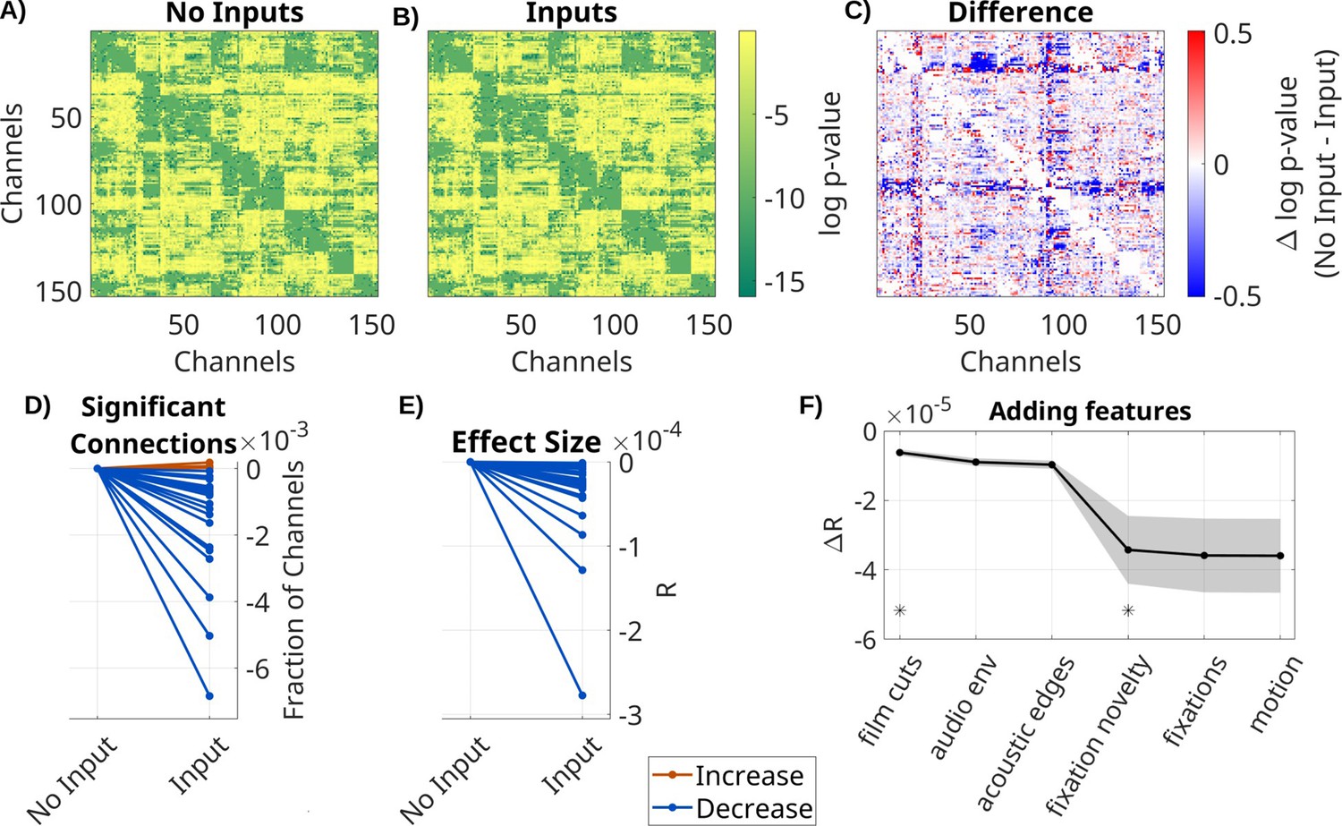
Spurious recurrent connectivity in A is removed when modeling the effect of extrinsic input with B.
Comparison of VARX model with and without inputs. (A) log p-values for each connection in A for a VARX model without inputs on one patient (Pat_1); (B) for a VARX model with inputs; (C) difference of log p-values for VARX model without minus with inputs (panels A and B). Both models are fit to the same data. (D) Thresholding panels A and B at p < 0.0001 gives a fraction of significant connections. Here, we show the fraction of significant channels for models with and without input. Each line is a patient with color indicating increase or decrease. (E) Mean over all channels for VARX models with and without inputs. Values in (D) and (E) have been normalized to models without input. (F) Change in R values when successively adding inputs to the VARX model. Black line shows mean across patients, shaded gray area the standard error of the mean. Stars indicate features that further reduce effect size over the previously added feature with statistical significance (Wilcoxon rank sum test p < 0.05). Negative values indicate a decrease in connectivity strength when the extrinsic inputs are accounted for. Results for broadband high-frequency activity (BHA) are shown in Figure 1—figure supplement 2.
Figure 1—figure supplement 1
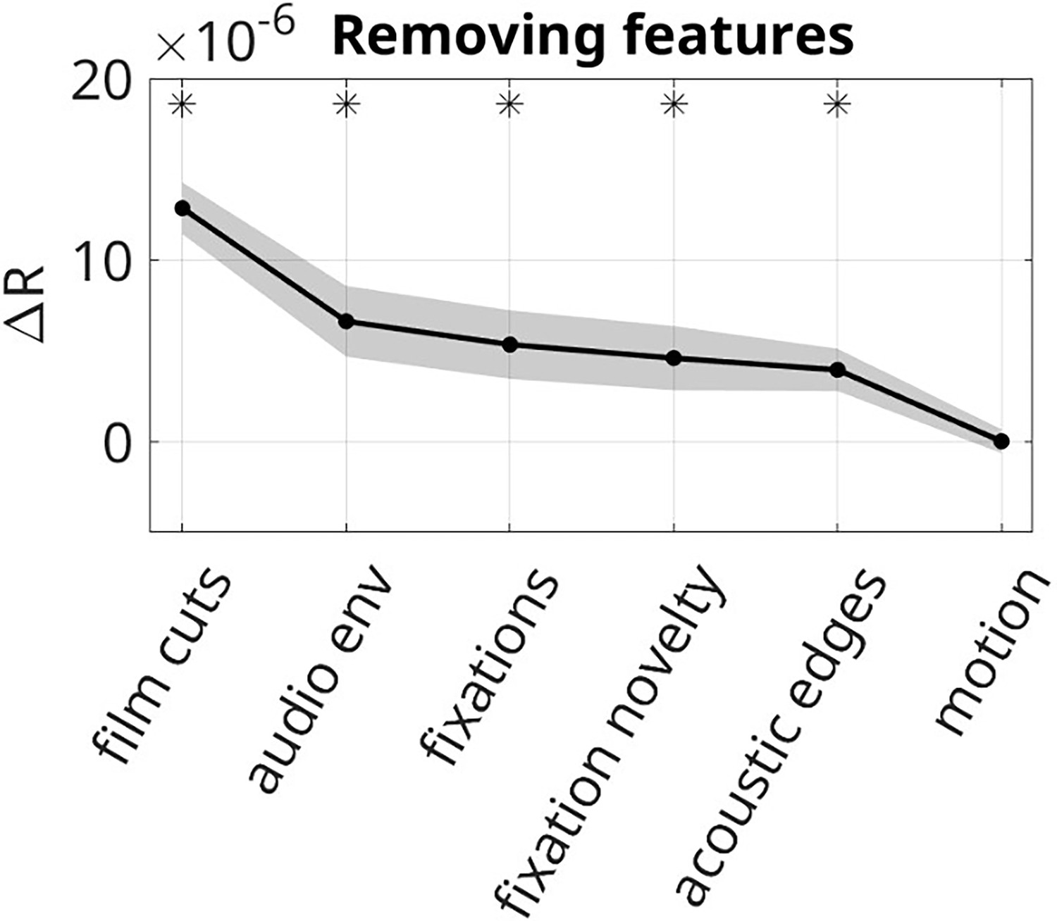
Effect of individual extrinsic features on effect size of recurrent connections.
Removing regressors for film cuts (ΔR = −12.8 × 10⁻⁶, p < 0.0001, N = 26), the auditory envelope (ΔR = −6.63 × 10⁻⁶, p = 0.0002, N = 26), fixation onset (ΔR = −5.6 × 10⁻⁶, p = 0.0009, N = 26), fixation novelty (ΔR = −4.6 × 10⁻⁶, p = 0.005, N = 26), or acoustic edges (ΔR = −3.95 × 10⁻⁶, p = 0.007, N = 26) significantly increases the effect size compared to the VARX model including all features. Removing the motion regressor does not show this effect (ΔR = −0.02 × 10⁻⁶, p = 0.64, N = 26). FDR correction, ɑ = 0.05. Black line shows the mean increase of effect size ΔR. Gray shaded area shows the standard error of the mean of ΔR across 26 patients. Stars indicate significant changes in effect size.
Figure 1—figure supplement 2
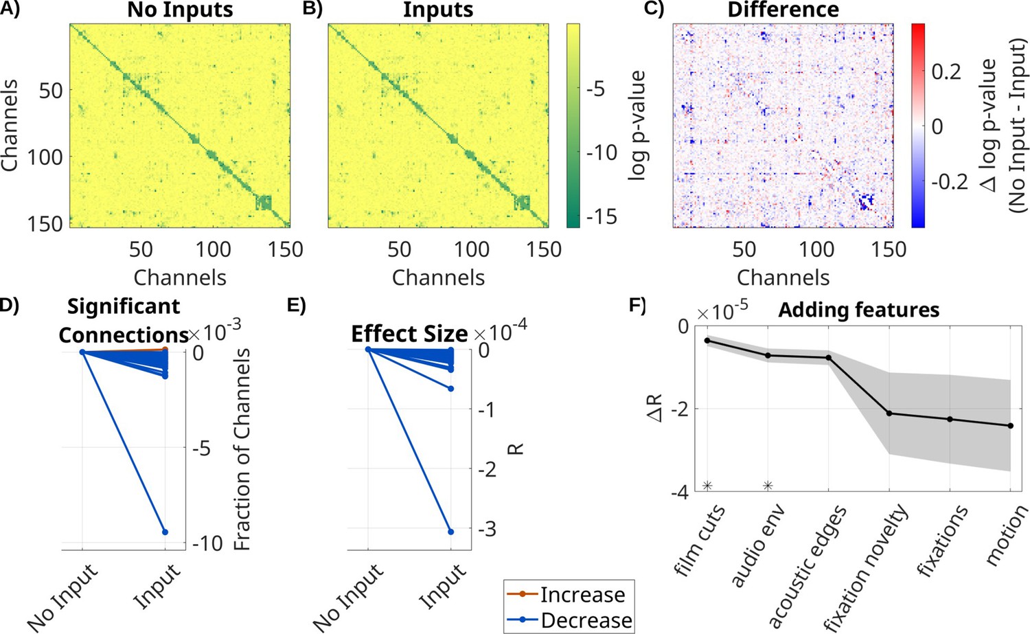
Spurious recurrent broadband high-frequency activity (BHA) connectivity in A is accounted for when modeling the effect of input with B.
Same analysis as in Figure 1 with BHA data. (A) log p-values for each connection in VARX model without inputs on one patient (Pat_1); (B) for VARX model with inputs; (C) difference. Both models are fit to the same data. (D) Fraction of significant recurrent connections in VARX models with and without inputs (difference: median = −3.7 × 10⁻⁴, p < 0.0001, N = 26, Wilcoxon). (E) Effect size R over all electrodes between VARX models with and without inputs (difference: median = −1 × 10⁻⁵, p < 0.0001, N = 26, Wilcoxon). Each line is a patient, with color indicating an increase or decrease. Values in (D) and (E) have been normalized to models without input. (F) Difference between the VARX model without input and VARX models successively adding inputs. Black line shows mean across patients, shaded gray area the standard error of the mean. Stars indicate features that further reduce effect size over the previously added feature with statistical significance (Wilcoxon rank sum test p < 0.05). Negative values indicate a decrease in connectivity strength when the extrinsic inputs are accounted for. Adding film cuts (ΔR = −3.6 × 10⁻⁶, p < 0.0001, N = 26, FDR correction, ɑ = 0.05) and the auditory envelope (ΔR = −3.6 × 10⁻⁶, p = 0.002, N = 26, FDR correction, ɑ = 0.05) significantly decrease R values.
Figure 2 with 3 supplements
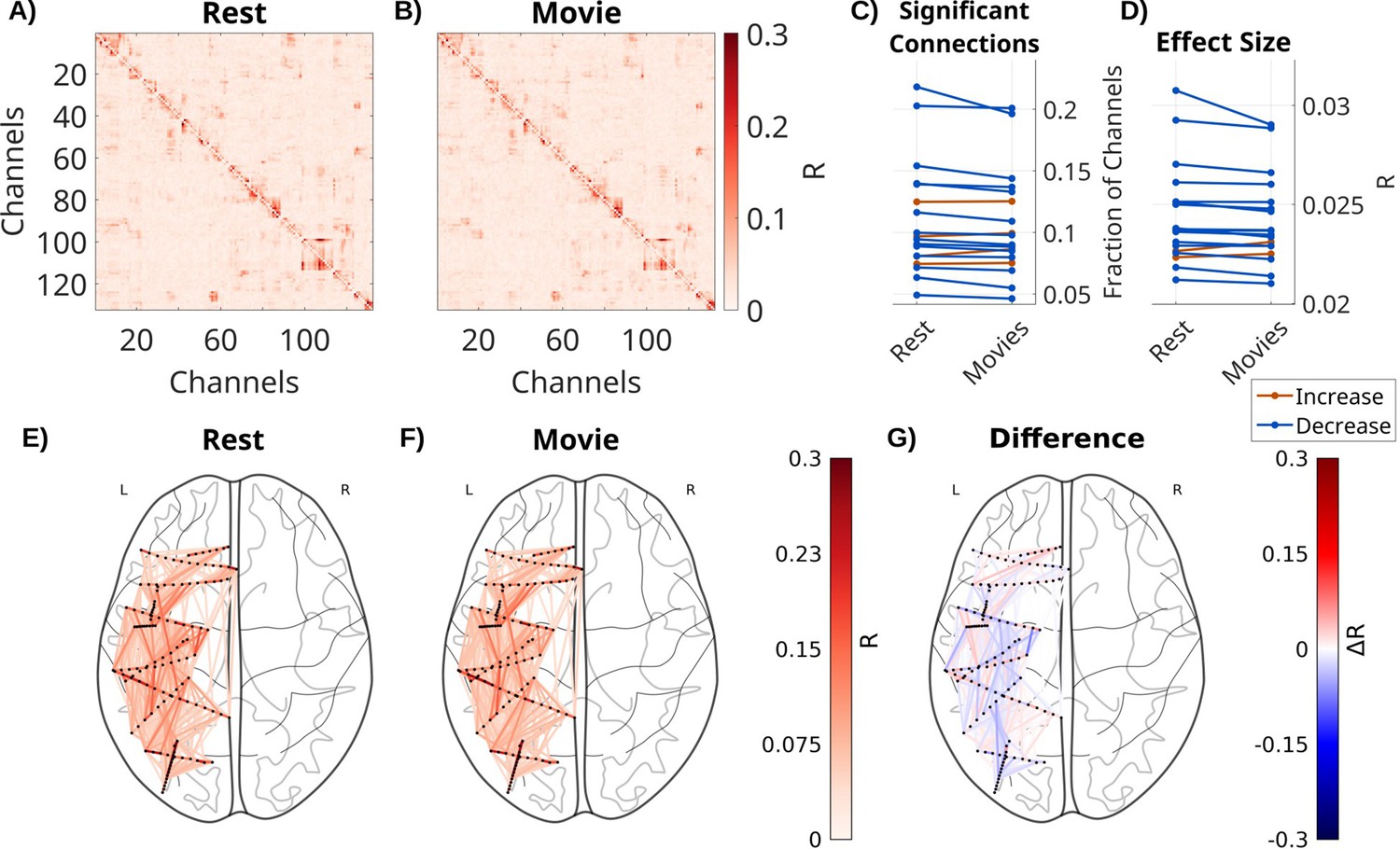
Recurrent connectivity during movies is decreased compared to rest.
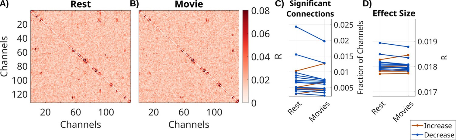
Effect size R for each connection in A for one patient (Pat_7) for (A) a VARX model during resting fixation with fixation onset as input feature. (B) The same with a VARX model of local field potential (LFP) recordings during movie watching, with the following input features: sound envelope, acoustic edges, fixation onsets, fixation novelty, motion, and film cuts. (C) Fraction of significant connections (p < 0.0001) for movies and rest. (D) Mean effect size across all channels for movies and rest. Each line is a patient, with color indicating a numerical increase or decrease. For the movie conditions, we averaged across four different 5-min movie segments. (E) Axial view of significant connections in resting state. Black dots show the location of contacts in MNI space. Lines show significant connections between contacts (p < 0.001) colored in red according to effect size R. For plotting purposes, connections in the upper triangle are plotted, and asymmetries are ignored. (F) The same for the movie task, and (G) the difference between movies and resting state, showing both increases and decreases for specific connections. Differences between broadband high-frequency activity (BHA) recurrent connectivity A during movies and resting state are shown in Figure 2—figure supplement 2.
Figure 2—figure supplement 1
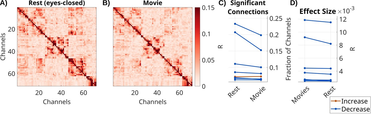
Recurrent connectivity decreases in movies compared to eyes-closed rest.
Effect size R for each connection in A in one patient (Pat_18_02) for (A) a VARX model of 5 min of local field potential (LFP) recordings during movie watching, with sound envelope, acoustic edge, fixation onsets, and novelty, motion, and film cuts as input features. (B) VARX model during eyes-closed rest without input features. Notably, the majority of electrodes in this patient are located in the occipital cortex. (C) The number of significant connections (p < 0.0001) across all patients is lower during movie watching (median = −0.0017, p = 0.01, N = 8, Wilcoxon). (D) Mean effect size across all channels is lower during movie watching (median = −0.0045, p = 0.02, N = 8, Wilcoxon). Each line represents one patient.
Figure 2—figure supplement 2
Recurrent connectivity A of broadband high-frequency activity (BHA) decreases during movie watching compared to rest.
Same analysis as in Figure 2 with BHA data. Effect size R for (A) a VARX model during resting fixation with fixation onset as input feature. (B) VARX model during movie watching, with sound envelope, acoustic edges, fixation onset and novelty, film cuts, and motion as input features. (C) Number of significant connections between movie and rest (fixed effect of stimulus: beta = –5.4 × 10⁻⁴, t(88) = –2.1, p = 0.042). (D) Mean effect size across all channels between movie and rest (fixed effect of stimulus: beta = –2.5 × 10⁻⁵, t(88) = –2.4, p = 0.17). Each line represents one patient.
Figure 2—figure supplement 3
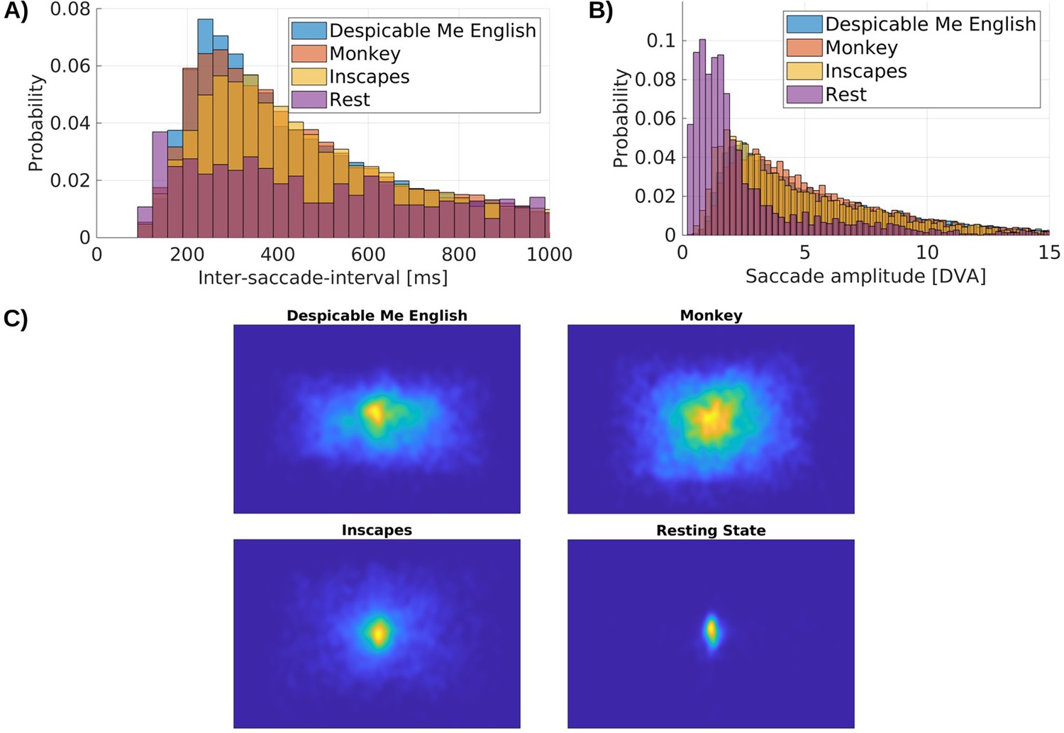
Eye movement behavior differs between movies and resting state.
(A) Normalized histogram of inter-saccade interval, the time between consecutive saccades. (B) Normalized histogram of saccade amplitude. (C) Heatmaps of fixation position for different recordings. All figures are based on 10 min of data for ‘Despicable Me English’, ‘Monkey’, and ‘Inscapes’ and 5 min of resting state. ‘Despicable Me English’: N = 13,643 saccades across 24 patients, with one recording each; ‘Monkey’: N = 12,790 saccades across 23 patients, with up to two recordings; ‘Inscapes’: N = 8562 saccades across 20 patients, with one recording each; ‘Rest’: N = 1510 saccades across 22 patients, with one recording each.
Figure 3 with 3 supplements

Impulse response models.
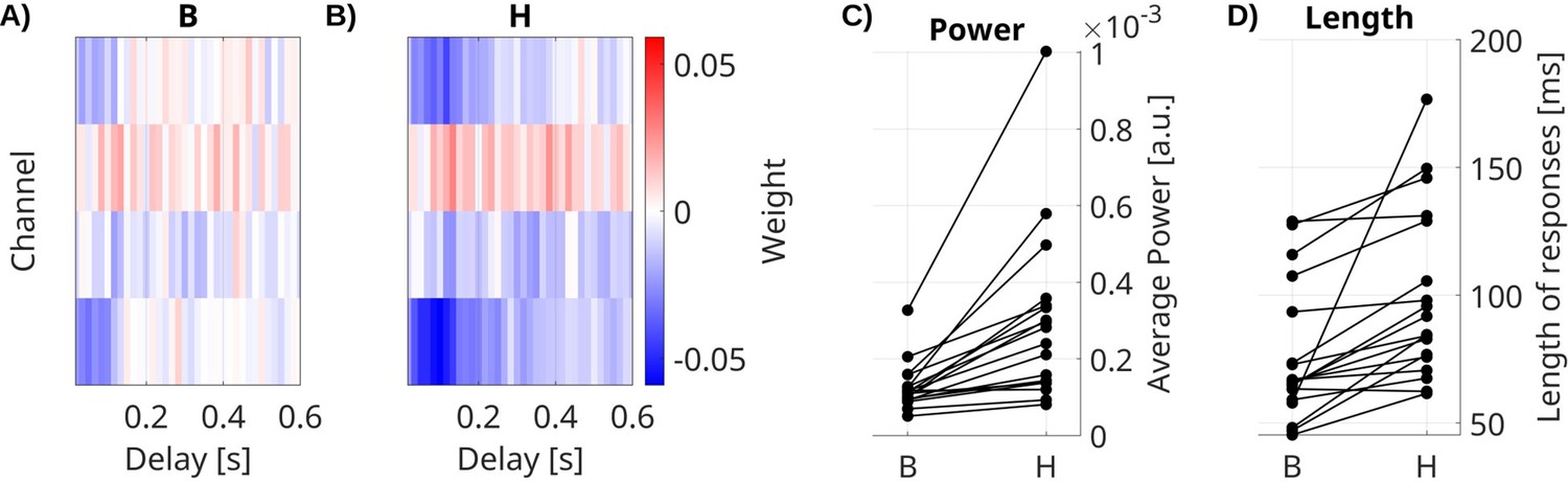
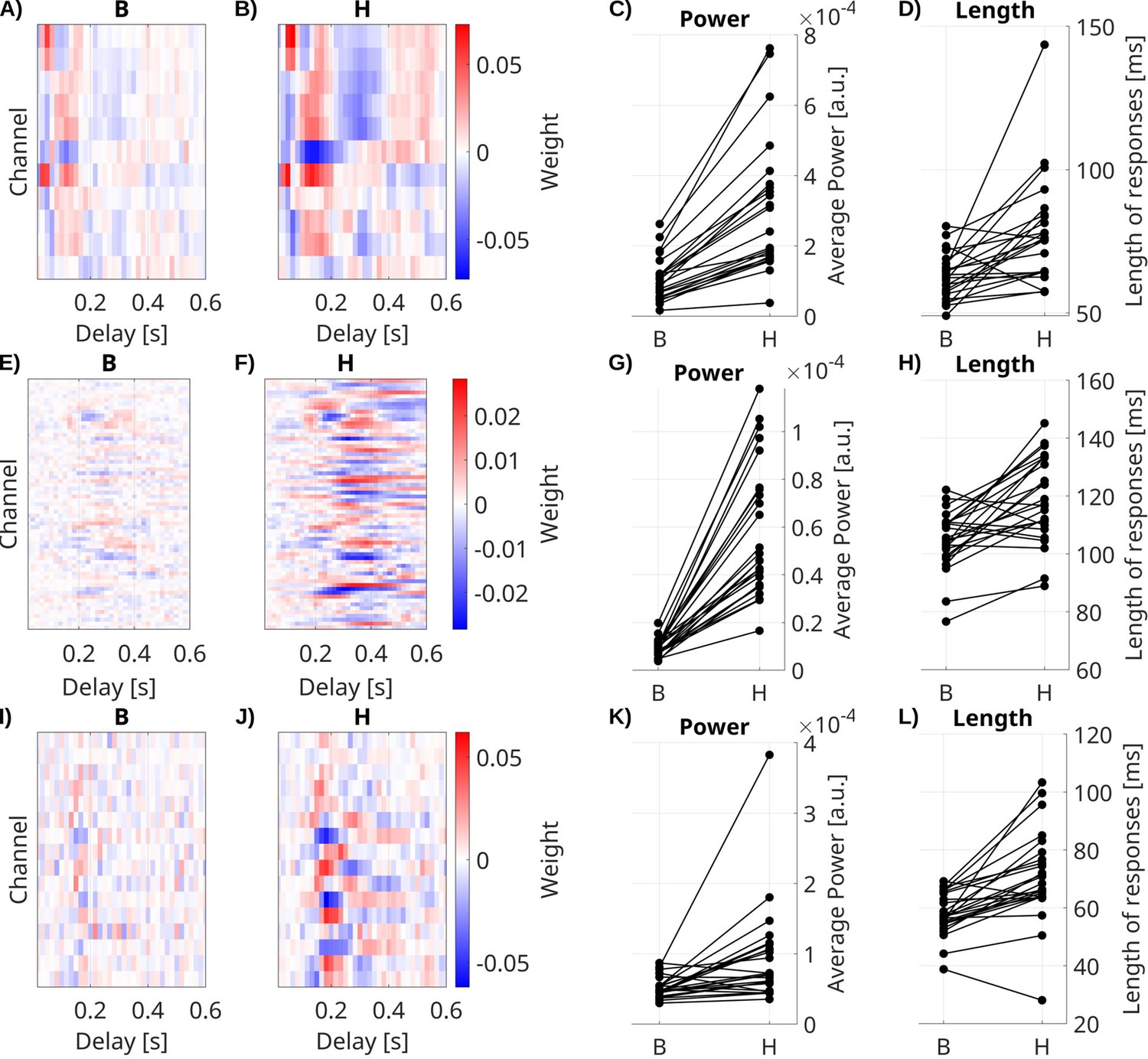
(A) Feed-forward responses B to fixation onset are weaker and shorter than (B) the overall system response H. Impulse response models for fixation onset in channels with significant responses for one example patient. (C) Power and (D) mean length of responses in significant channels for all patients. Each line is a patient. Responses to fixation onset in all significant channels, as well as auditory envelope and film cuts, are shown in Figure 3—figure supplement 2.
Figure 3—figure supplement 1
Broadband high-frequency activity (BHA) impulse response models.
(A) Feed-forward BHA responses B to fixation onset are weaker and shorter than (B) the overall system response H. Significant responses for Pat_1. (C) Power of responses B is weaker than H (medianΔ = −1.3 × 10⁻⁴, p = 0.0002, N = 18, Wilcoxon). (D) Mean length of responses B is shorter than H (medianΔ = −17.50 ms, p = 0.0002, N = 18, Wilcoxon). Each line represents average values across significant channels in a patient.
Figure 3—figure supplement 2
Impulse response models.
Input responses to fixations onset (A–D), film cuts (E–H), and auditory envelope (I–L). Feed-forward responses B (A, E, I) are weaker and shorter than the overall system response H (B, F, J). Significant responses for Pat_1. Power of responses to fixation onset B is weaker than H for (C) fixation onset (medianΔ = −1.5 × 10⁻⁴, p < 0.0001, N = 23, Wilcoxon), (G) film cuts (medianΔ = −3.9 × 10⁻⁵, p = 0.0001, N = 25, Wilcoxon), and (K) auditory envelope (medianΔ = −2.3 × 10⁻⁵, p = 0.0004, N = 25, Wilcoxon). Mean length of responses to fixation onset B is shorter than H for (D) fixation onset (medianΔ = −10.9 ms, p < 0.0001, N = 23, Wilcoxon), (H) film cuts (medianΔ = −14.98 ms, p = 0.0002, N = 25, Wilcoxon), (L) and auditory envelope (medianΔ = −10.53 ms, p < 0.0001, N = 25, Wilcoxon). Each line represents average values across significant channels in a patient.
Figure 3—figure supplement 3
Robustness of estimates of input filters B to intrinsic effects and uncorrelated features.
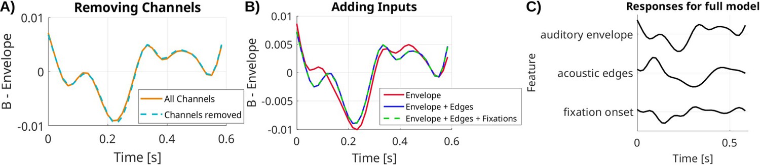
(A) Removing half of all channels that do not show responses to the auditory envelope does not change the estimate of the response filter B. (B) The estimate of the responses B to the auditory envelope (red line) is changed by adding a correlated feature (acoustic edges, blue line), but not by adding an uncorrelated feature (fixation onset, green dashed line). (C) The example channel shown in panels A and B shows responses to the auditory envelope, acoustic edges, and fixation onset. For clearer visualization purposes, responses have been filtered with a 10-Hz low-pass filter.
Figure 4
For broadband high-frequency activity (BHA), relative power of innovation versus signal drops during movies as compared to rest in responsive channels.
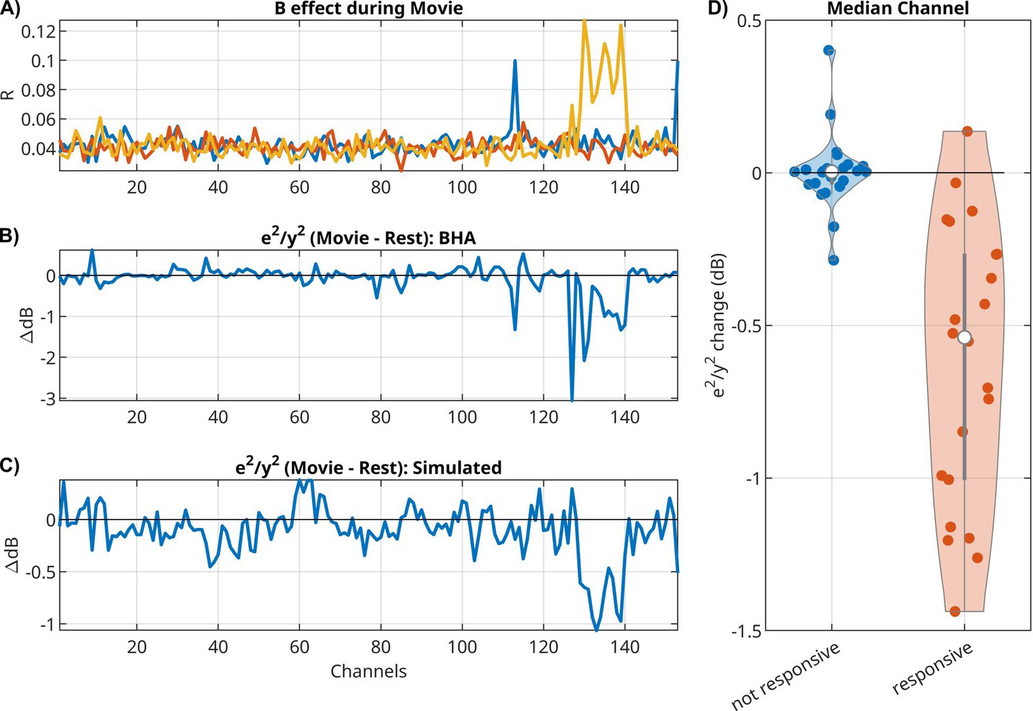
(A) Effect size R for extrinsic effect B in all channels for three input features (scene cuts, fixation onset, and sound envelope). In this example, 15 electrodes had significant responses to one of the three inputs (Bonferroni corrected at p < 0.01). (B) Change in relative power of innovation (dB(innovation power/signal power), then subtracting movie − rest). (C) Change in relative power of innovation in a simulation of a VARX model with gain adaptation. Here, we are using the A and B filters that were estimated on BHA on the example from panels A and B. (D) Median of power ratio change across all patients, contrasting responsive versus non-responsive channels.
Figure 5 with 1 supplement
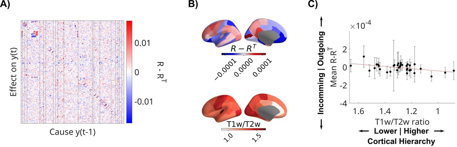
Recurrent connectivity of local field potential (LFP) is directed from sensory to higher-order areas.
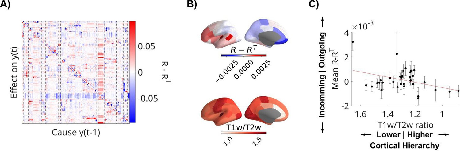
(A) Difference of R-RT showing asymmetric directed effects. Dashed lines indicate regions of interest in the Desikan–Killiany atlas. (B) Mean directionality across patients and T1w/T2w ratio are averaged in parcels of the Desikan–Killiany atlas. (C) Mean directionality is correlated with cortical hierarchy, estimated with the T1w/T2w ratio. Each dot represents a parcel in the Desikan–Kiliany atlas with error bars indicating error of the mean across patients with channels in that parcel. The datapoint on the top left is the transverse temporal gyrus. Note that the x-axis has been flipped to show areas higher on the cortical hierarchy on the right. T1w/T2w ratio and cortical hierarchy have an inverse relationship.
Figure 5—figure supplement 1
Directionality of recurrent broadband high-frequency activity (BHA) connectivity in relation to cortical hierarchy.
Analysis as in Figure 5. (A) Difference of R-RT showing asymmetric directed effects. Dashed lines indicate regions of interest in the Desikan–Killiany atlas. (B) Mean directionality across patients and T1w/T2w ratio are averaged in parcels of the Desikan–Killiany atlas. (C) Mean directionality is not significantly correlated with cortical hierarchy, estimated with the T1w/T2w ratio (t(533) = 2.19, p = 0.029).
Figure 6
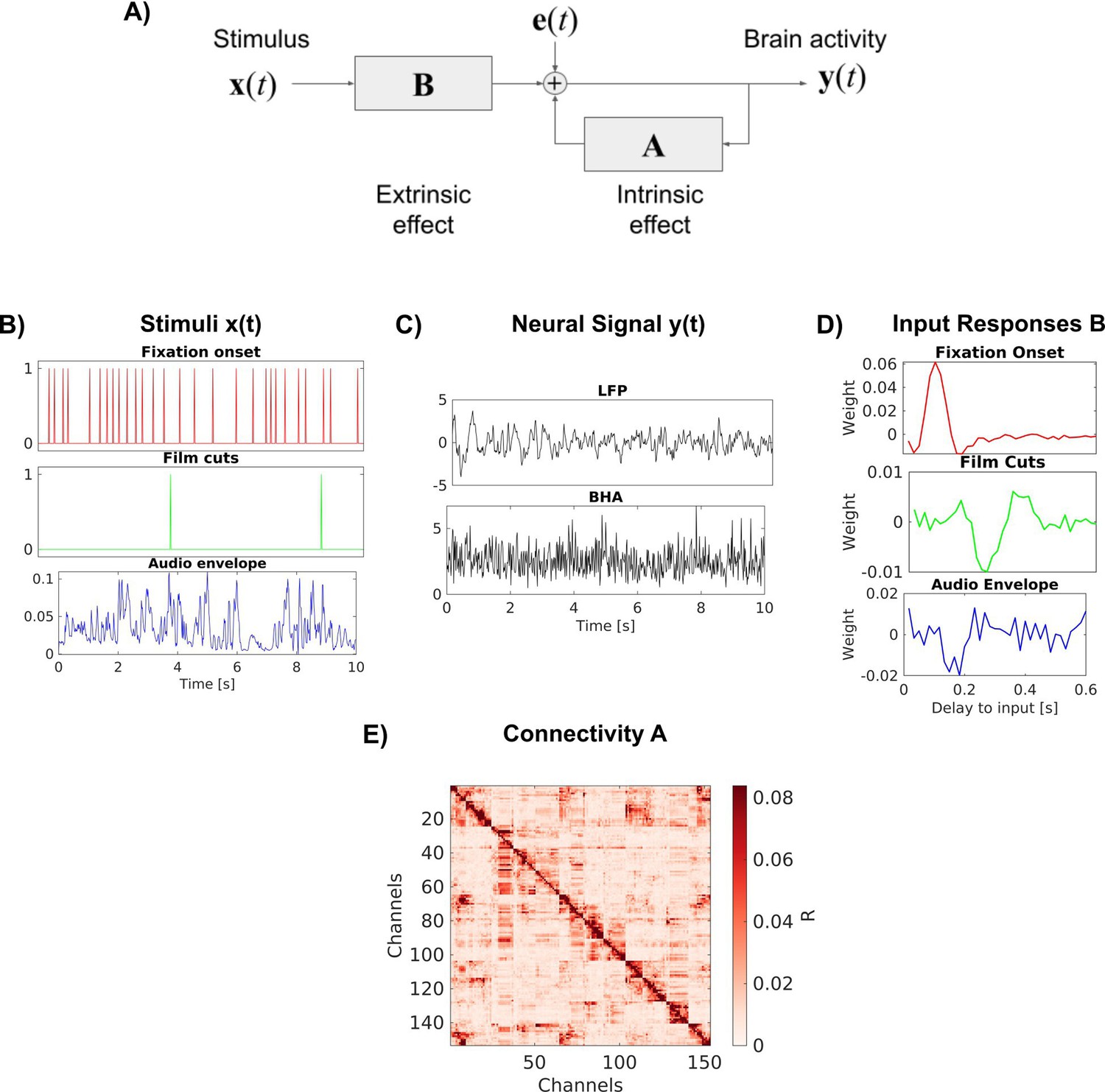
VARX model of the brain.
(A) Block diagram of the VARX model. y(t) represents observable neural activity in different brain areas, x(t) are observable features of a continuous sensory stimulus, A represents the recurrent connections within and between brain areas (intrinsic effect), and B captures the transduction of the sensory stimuli into neural activity and transmission to different brain areas (extrinsic effect). The diagonal term in A captures recurrent feedback within a brain area. Finally, e(t) captures unobserved ‘random’ brain activity, which leads to intrinsic variability. (B) Example of input stimulus features x(t). (C) Example of neural signal y(t) recorded at a single location in the brain. We analyze local field potentials (LFPs) and broad-band high-frequency activity (BHA) in separate analyses. (D) Examples of filters B for individual feed-forward connections between an extrinsic input and a specific recording location in the brain. (E) Effect size R for the recurrent connections captured by auto-regressive filters A.
Figure 7 with 2 supplements
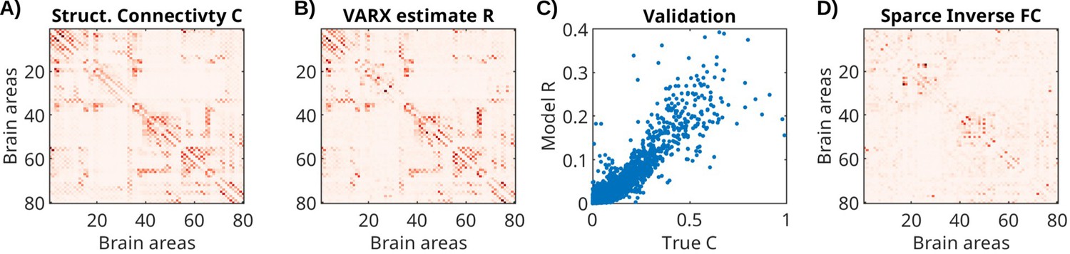
Structural connectivity of stimulated neural mass model for the whole brain, and estimated recurrent connectivity in VARX model.
(A) True structural connectivity C used to simulate neural activity using a neural mass model with the neurolib python toolbox. Structural connectivity is based on diffusion tensor imaging data between 80 brain areas (called Cmat in neurolib). Here showing the square root of the ‘Cmat’ matrix for better visibility of small connectivity values. (B) Effect size estimate R for the recurrent connectivity matrix A of the VARX model on the simulated data. The diagonal in R is omitted as it is also missing in the structural connectivity Cmat. (C) Comparison of true and VARX estimate of connectivity. (D) Absolute value of the sparse-inverse functional connectivity (estimated using graphical lasso Friedman et al., 2008).
Figure 7—figure supplement 1
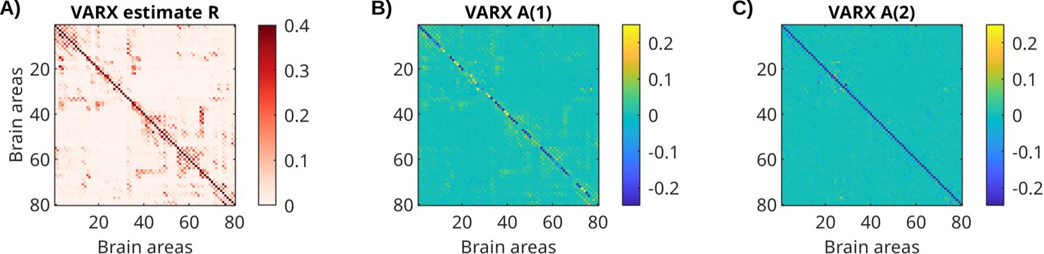
Connectivity of stimulated neural mass model.
(A) Same effect size matrix R as in Figure 7B, except now the diagonal element is shown. Filter matrix A for (B) delay 1 and (C) delay 2. The color axis has been limited to ±0.25 for visibility of off-diagonal elements.
Figure 7—figure supplement 2
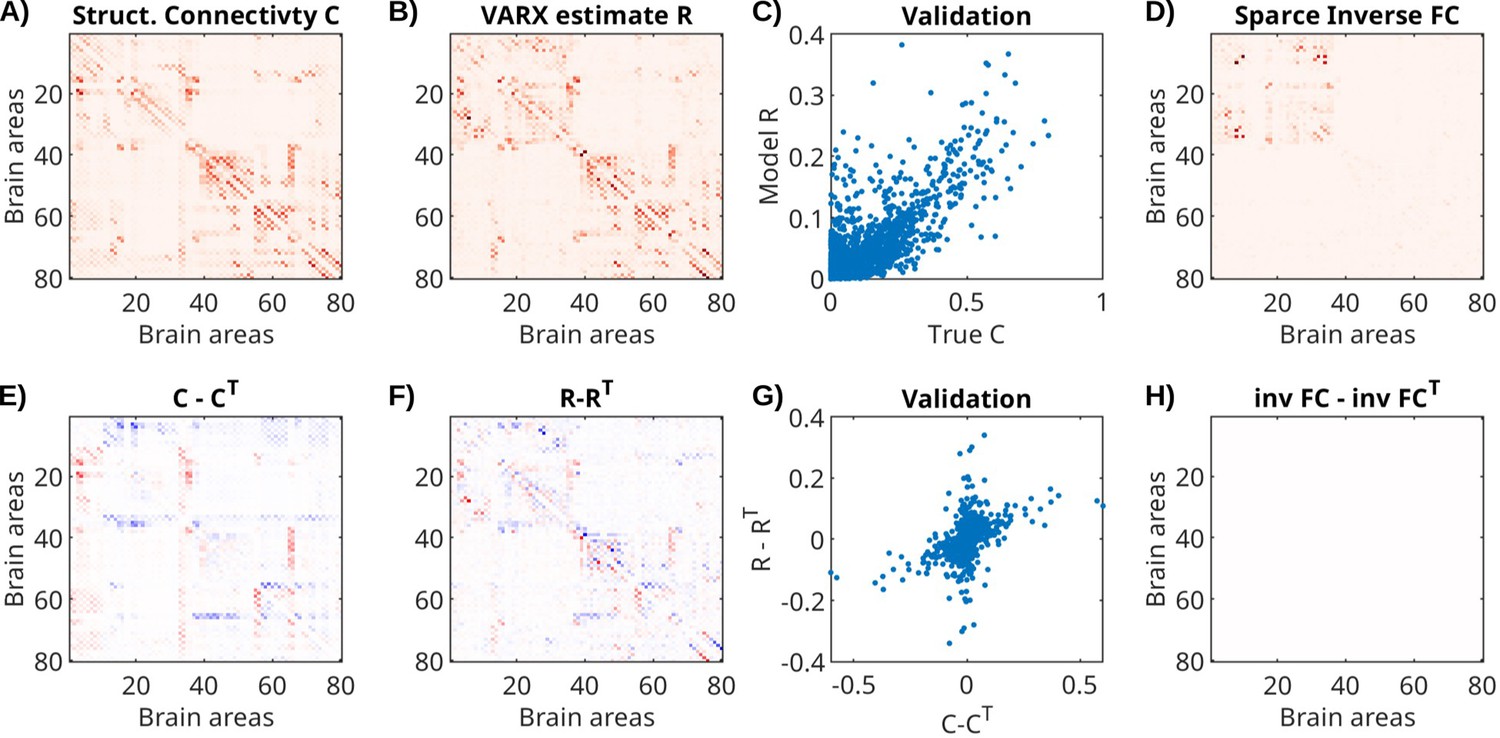
Connectivity of stimulated neural mass model with asymmetric structural connectivity.
(A) Same as in Figure 7A, however, rows 1:10, 65:66, 33:36, and 55:56 have been downscaled by a factor of 0.1 to enhance the asymmetry of the structural connectivity matrix for nodes that had larger connectivity between distant brain areas. Note again that the diagonal in R is omitted as it is also missing in the structural connectivity matrix of the simulation. (B) Effect size R for VARX model on updated simulated data. (C) Spearman correlation drops to r = 0.54 (from 0.69 in Figure 7). (D) Absolute value of the sparse-inverse functional connectivity on updated simulated data. (E) Asymmetry is highlighted by subtracting the transpose (same as in Figure 5). (F) The VARX largely recovers the sign of the asymmetry. (G) But a number of nodes are misestimated. (H) The sparse inverse covariance, by definition, is symmetric and does not capture any asymmetry.
Appendix 1—figure 1
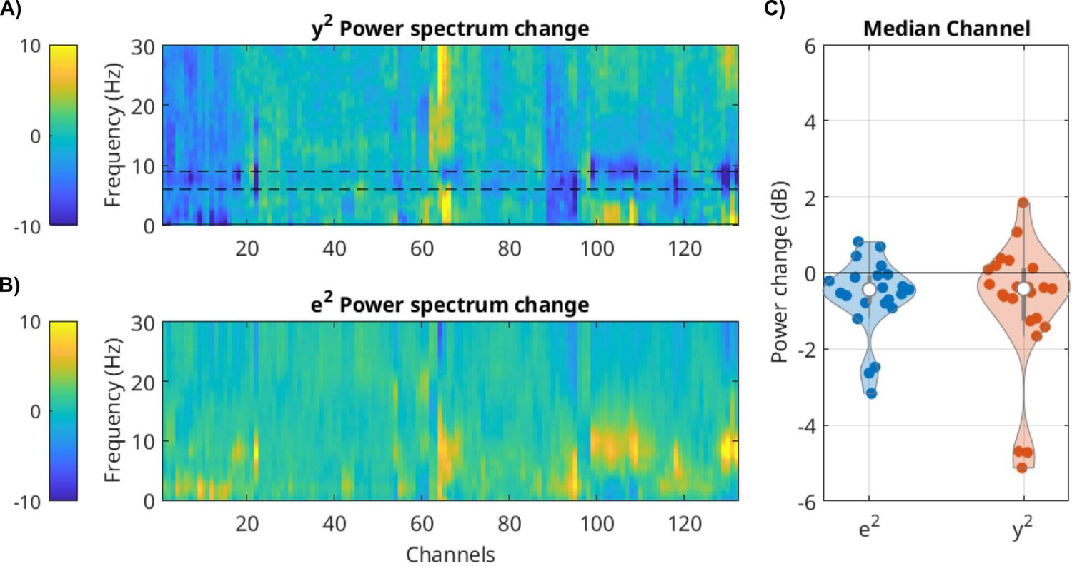
For local field potential (LFP), the power of the signal and innovation process drops during movies as compared to rest.
Difference in LFP power between movies minus rest. Negative values indicate stronger power during rest. (A) Difference in power spectrum for the raw signal y(t) for one patient. False color indicates change in the power spectrum in dB (blue hues indicate stronger power during rest). Dashed black lines bracket 5 and 11 Hz. (B) Difference in power spectrum for the innovation process e(t). (C) Power difference movie minus rest for each of 25 patients (each point is the median over channels).
Appendix 1—figure 2
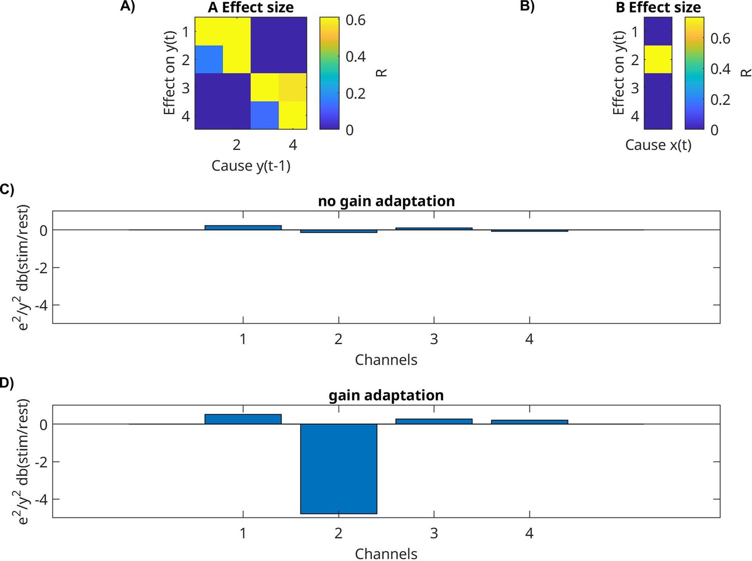
Gain adaptation on a toy example.
In this small recurrent network, there are four nodes, with each of two nodes connected. Input only arrives at one node. Data are simulated with and without gain adaptation and then estimated with the VARX model. (A) Estimated recurrent connectivity. (B) Estimated input connectivity estimated during ‘stimulus’ condition. Relative power of the innovation e(t) (relative to signal y(t)) subtracting dB between stimulus − rest condition, (C) without and (D) with gain adaptation. ‘Rest’ here means that the input x(t) was zero.
Appendix 3—figure 1
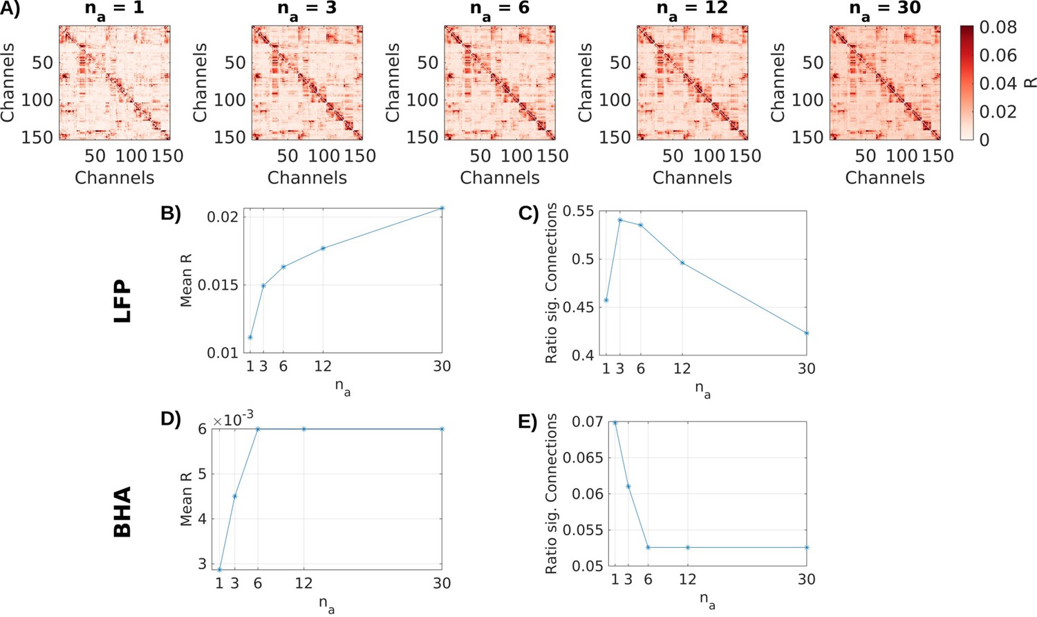
Choice of na.
(A) Effect size R of connections in local field potential (LFP) data for an example patient using different values for the delays na. (B) Mean effect size R and (C) ratio of significant (p < 0.001) channels across all channels for different na for LFP data. (D) and (E) in broadband high-frequency activity (BHA).
Tables
Table 1
Models commonly used in neural signal analysis.
(a) ‘Interact’ refers to an additional bilinear interaction term of the form x C y that allows for a modulation of intrinsic effect by the external input. (b) The DCM is defined in terms of the first derivative of y(t), which in discrete time is the same as na = 1. (c) It is straightforward to add an interaction term to the VARX model and maintain fast OLS estimation.
| Model | Intrinsic effect A | Extrinsic effect B | Interact | Delayna,, nb | Estimation speed | Reference, with code where available |
|---|---|---|---|---|---|---|
| GLM | No | Yes | No | = 1 | Medium | Friston et al., 1994, SPM, FSL |
| DCM | Yes | Yes | Yesa | = 1b | Slow | Friston et al., 2003, no code |
| VAR | Yes | No | No | >1 | Fast/slow | Barnett and Seth, 2014 |
| mTRF | No | Yes | No | >1 | Fast | Crosse et al., 2016 |
| VARX | Yes | Yes | Noc | >1 | Fast | Parra et al., 2025 |
Appendix 2—table 1
Demographics, length of recordings, and number of recording channels.
Data from patients 9, 11, 18, and 23 were recorded from two reimplants each at different times.
| Patient ID | Age | Sex | Total length of recordings [min] | Number of channels |
|---|---|---|---|---|
| Pat_1 | 58 | M | 58.6 | 153 |
| Pat_2 | 22 | M | 48.6 | 164 |
| Pat_5 | 48 | M | 58.6 | 334 |
| Pat_6 | 36 | F | 58.6 | 189 |
| Pat_7 | 43 | M | 58.6 | 132 |
| Pat_8 | 41 | F | 64.7 | 154 |
| Pat_9 | 50 | M | 58.6 | 267 |
| Pat_9_02 | 51 | M | 58.6 | 271 |
| Pat_10 | 24 | M | 53.6 | 192 |
| Pat_11 | 37 | M | 58.6 | 192 |
| Pat_11_02 | 37 | M | 58.6 | 111 |
| Pat_12 | 52 | F | 48.6 | 198 |
| Pat_13_02 | 24 | M | 58.6 | 296 |
| Pat_14 | 20 | M | 58.6 | 207 |
| Pat_15 | 56 | M | 53.6 | 100 |
| Pat_16 | 43 | F | 39.3 | 261 |
| Pat_17 | 27 | F | 58.6 | 220 |
| Pat_18 | 28 | F | 58.6 | 227 |
| Pat_18_02 | 30 | F | 58.6 | 71 |
| Pat_19 | 46 | M | 48.6 | 230 |
| Pat_20 | 35 | F | 54.3 | 231 |
| Pat_21 | 48 | M | 58.6 | 323 |
| Pat_22 | 19 | M | 48.6 | 75 |
| Pat_23 | 36 | F | 54.4 | 175 |
| Pat_23_03 | 36 | F | 48.7 | 260 |
| Pat_24 | 59 | F | 39.3 | 60 |
Additional files
Download links
A two-part list of links to download the article, or parts of the article, in various formats.
Downloads (link to download the article as PDF)
Open citations (links to open the citations from this article in various online reference manager services)
Cite this article (links to download the citations from this article in formats compatible with various reference manager tools)
Intrinsic dynamic shapes responses to external stimulation in the human brain
eLife 14:RP104996.
https://doi.org/10.7554/eLife.104996.3


