A platform for brain-wide imaging and reconstruction of individual neurons
- Janelia Research Campus, Howard Hughes Medical Institute, United States
- National Institute of Mental Health, United States
- Max Planck Institute of Molecular Cell Biology and Genetics, Germany
Figures
Figure 1 with 1 supplement
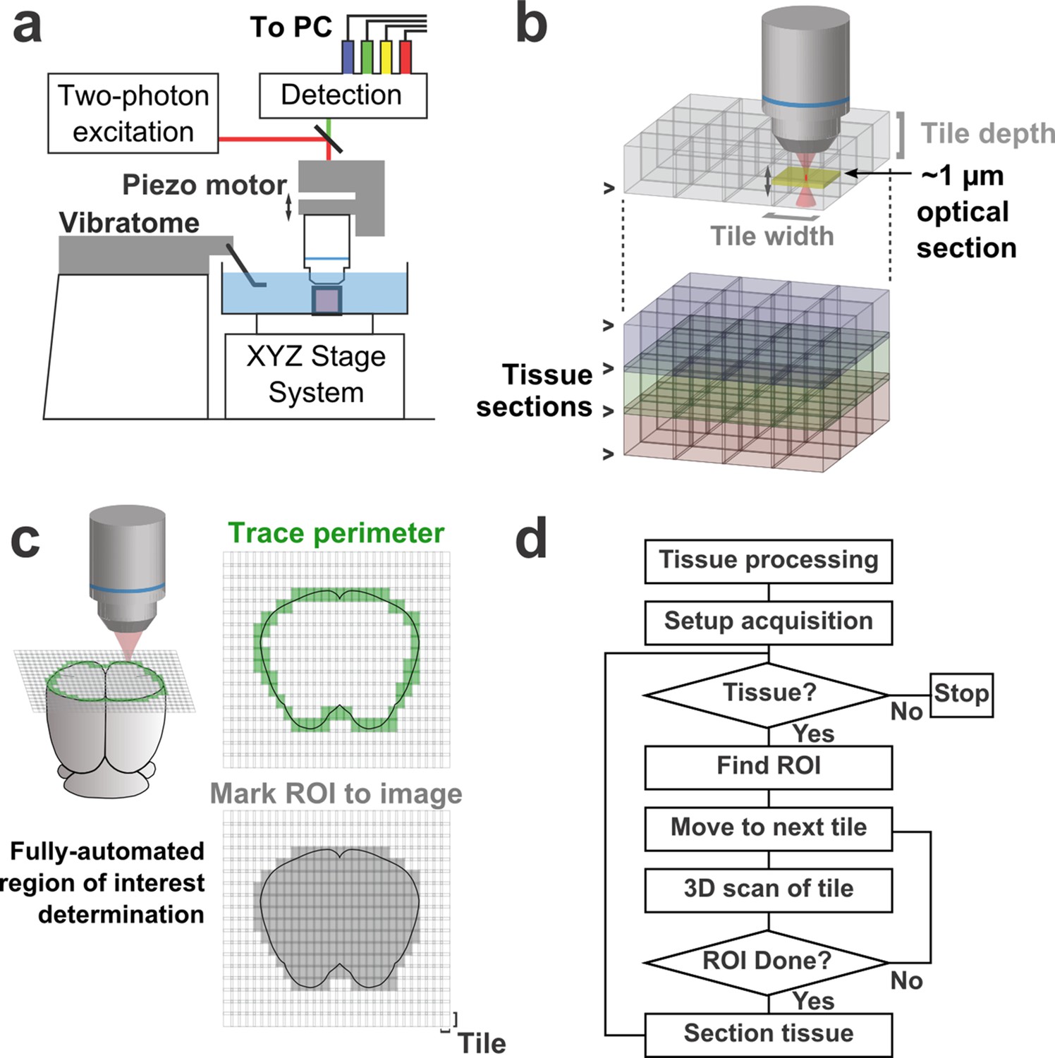
Schematic of imaging system.
(a) Schematic of apparatus for automated volumetric two-photon tomography. (b) To image large volumes of tissue, a collection of three-dimensional image stacks (tiles) covering the full volume of the tissue sample was acquired serially. Tiles overlapped in all three dimensions to aid in image registration and ensure coverage of the full volume. (c) The active imaging region is determined for each section by first tracing the perimeter of the tissue block and then filling in any tiles internal to the traced region. (d) Flow chart illustrating the tasks performed during data acquisition.
Figure 1—figure supplement 1

Point spread function measurement.
(a) Empirically-measured point spread function measured using 200-nm fluorescent polystyrene beads.
Figure 2
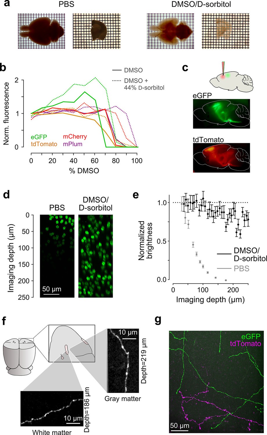
Sample preparation and clearing.
(a) Whole brains (left) and 1 mm-thick tissue sections (right) cleared using dimethyl sulfoxide (DMSO) and d-sorbitol. (b) Fluorescence of purified eGFP as a function of DMSO concentration (v/v) in 10 mM HEPES, pH 7.3 (open circles) and 10 mM HEPES, pH 7.3 containing 44% (w/v) d-sorbitol (filled circles). (c) eGFP and tdTomato fluorescence in a cleared hemi-brain demonstrates preservation of native fluorescence. (d) Maximum intensity projections of side views of image tiles of histone 2B-eGFP labeled nuclei from a DMSO/d-sorbitol cleared section (right) and from a matched section in phosphate buffered saline (PBS; left) from the contralateral hemisphere of the same brain. (e) Quantification of intensities of histone 2B-eGFP labeled nuclei as a function of depth (PBS: n=204 detected nuclei in two tiles; DMSO/d-sorbitol: n=815 detected nuclei in three tiles). (f) Representative images of a single axonal collateral as it passes through the anterior commissure (white) and surrounding olfactory cortex (gray). Images were acquired at a depth >180 μm in each case and scaled in the same manner. (g) Axons labeled with multiple fluorophores could be simultaneously imaged with high signal to noise within cleared tissue. Note that imaging fine axons through the axially oriented anterior commissure in this example represent a stringent test of clearing due to the high degree of optical scattering observed in white matter tracts. DMSO, dimethyl sulfoxide; eGFP, enhanced green fluorescent protein.
Figure 3 with 1 supplement
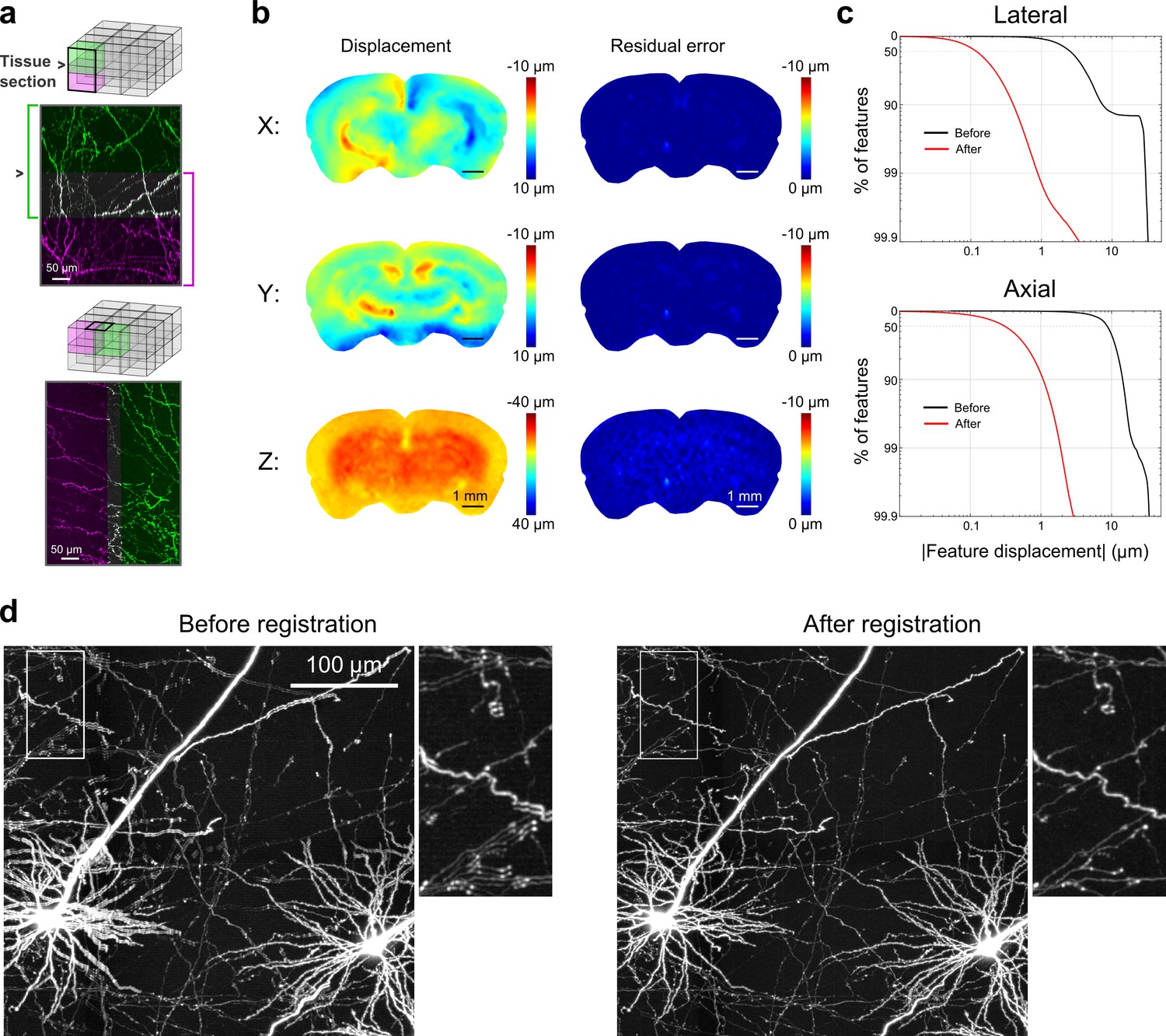
Registration of image tiles.
(a) Example registration of pairs of image tiles in the axial (left) and lateral (right) directions. (b) Initial displacement of automatically-identified features as a result of sectioning (left) across the full extent of the exposed tissue surface. Displacements along each Cartesian direction are displayed in separate heat maps for a representative section. Right: residual displacement of the same feature set after linear interpolation of displacements across each tile. (c) Distribution of the residual displacements of all features identified in a whole-brain dataset in the lateral (top) and axial (bottom) directions before (black) and after (red) image registration. (d) Maximum-intensity projection through a volume containing labeled neurons before (left) and after (right) the registration procedure.
Figure 3—figure supplement 1
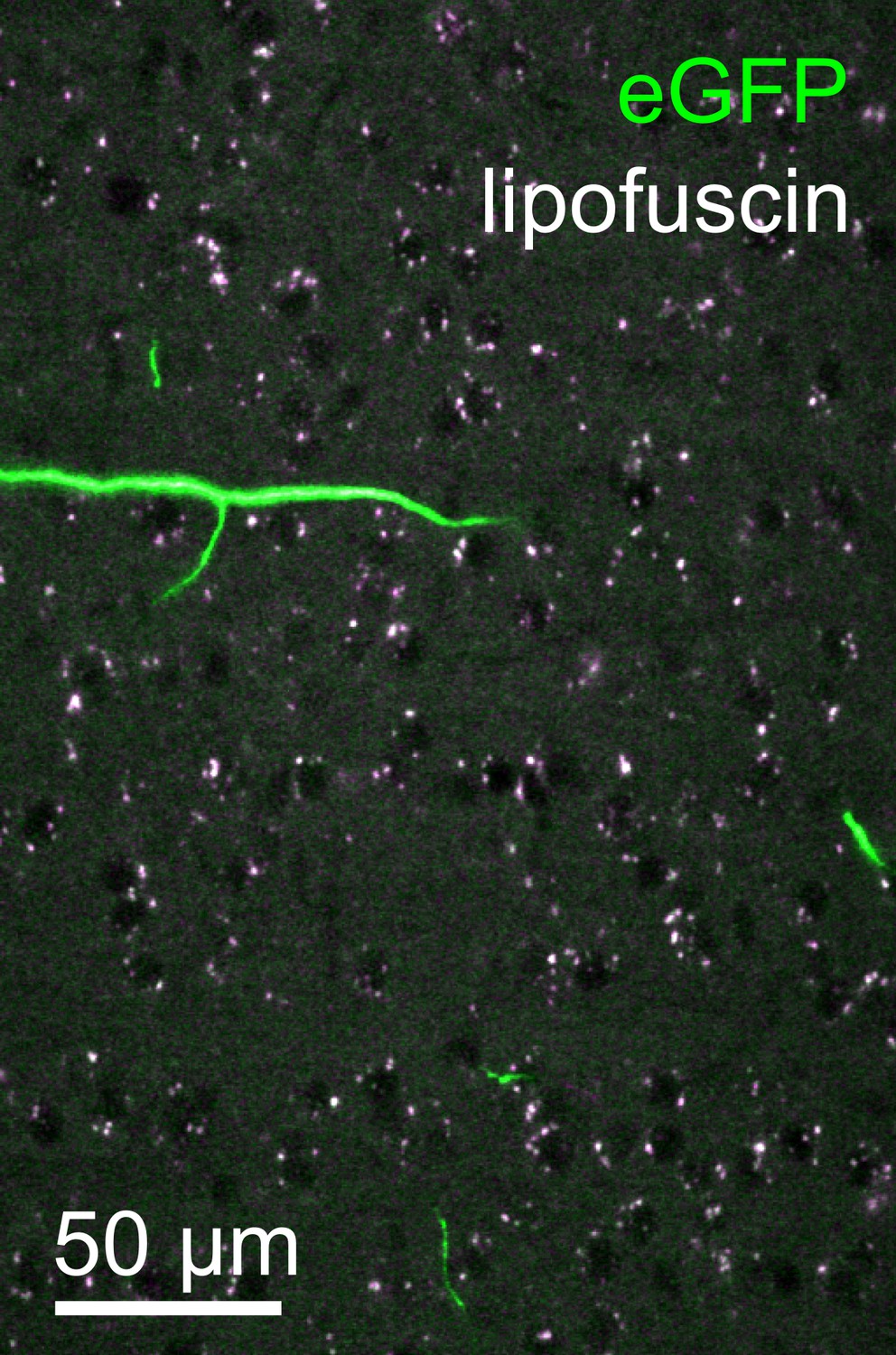
Lipofuscin imaging.
Overlay of fluorescence captured in the green (500–550 nm) and orange (580–653 nm) spectral bands from a representative tile within the neocortex. Autofluorescent lipofuscin (white puncta) could be imaged reliably. These features, present throughout the brain, were utilized for post hoc registration. Lipofuscin was easily distinguished from enhanced green fluorescent protein (eGFP)-labeled structures by its broad emission spectrum.
Figure 4 with 1 supplement
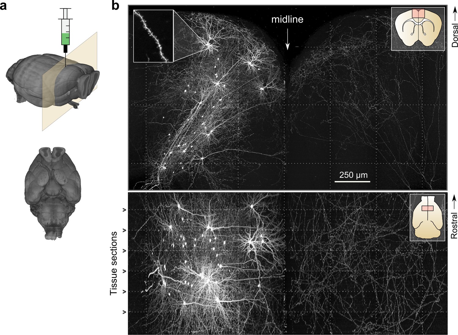
Whole-brain imaging.
(a) Three-dimensional rendering of complete mouse brain dataset as viewed from an anterolateral (left) and ventral (right) perspective. (b) Maximum intensity projection through a large tissue volume containing labeled somata and neurites in the X–Y (top) and X–Z (bottom) planes (2.3 × 1.3 × 1.0 mm). Axon collaterals are clearly discernible in the contralateral hemisphere despite the large volume of tissue depicted. Dotted lines represent borders between adjacent tiles. Insets (top right) represent the location and orientation of each image in relation to a coronal (top) and horizontal (bottom) section. Inset at top left illustrates detail in full-resolution images. Following registration of the full collection of tiles comprising a full dataset, individual neurites appear continuous between tiles separated in the axial direction (bottom; separated by a physical tissue section) while maintaining continuity in laterally adjacent tiles (top).
Figure 4—figure supplement 1

High speed, high-power imaging.
(a) Image of an axonal collateral with low (top) and high (bottom) excitation power. High-power imaging improves signal-to-noise without degrading resolution due to fluorophore saturation. (b) Peak-normalized fluorescence intensity along the cross sections indicated above in (a) resulting from low- (black) and high-power imaging (red).
Figure 5 with 1 supplement
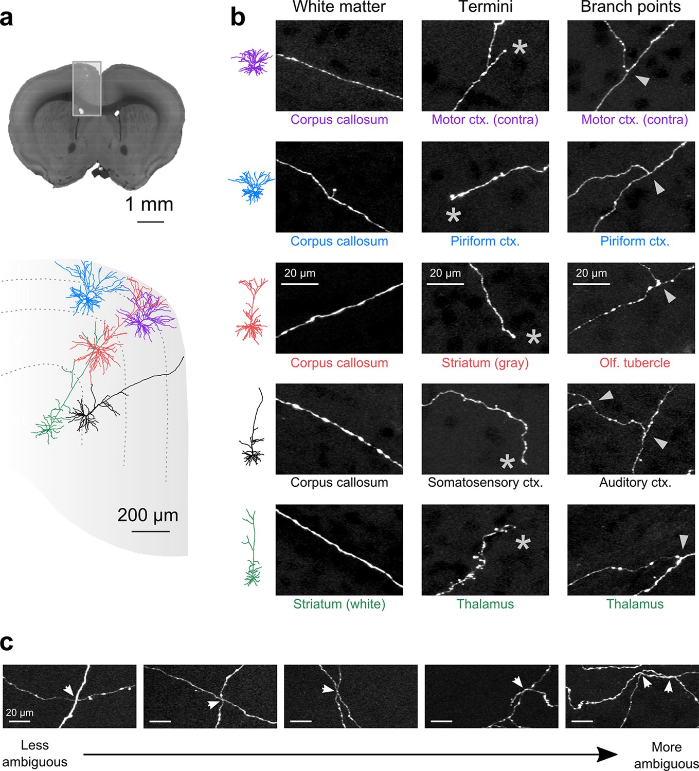
Axon collaterals are labeled with high signal-to-noise across their entire length.
(a) Top: Virtual coronal section through whole-brain dataset. Boxed area denotes region containing labeled somata and is expanded in schematic below. Bottom: Laminar distribution and dendritic morphology of five labeled neurons spanning layers II–VI. (b) Representative images of axonal segments from each of the five neurons in white matter (left), at branch points (middle; denoted by asterisks) and at termini (right; denoted by arrowheads). The location of each axonal segment is listed below the corresponding images, and in all cases, segments were in a different brain structure than their associated somata. All images are maximum intensity projections through a depth of 20 μm. (c) Regions with high labeling density contain axon crossovers that introduce ambiguity into axonal reconstruction. Examples of crossover points ordered subjectively by approximate degree of difficulty in assignment of segment identity. The two-dimensional examples shown here are for illustration purposes; ambiguity arises only when segments are closely apposed in all the three dimensions.
Figure 5—figure supplement 1
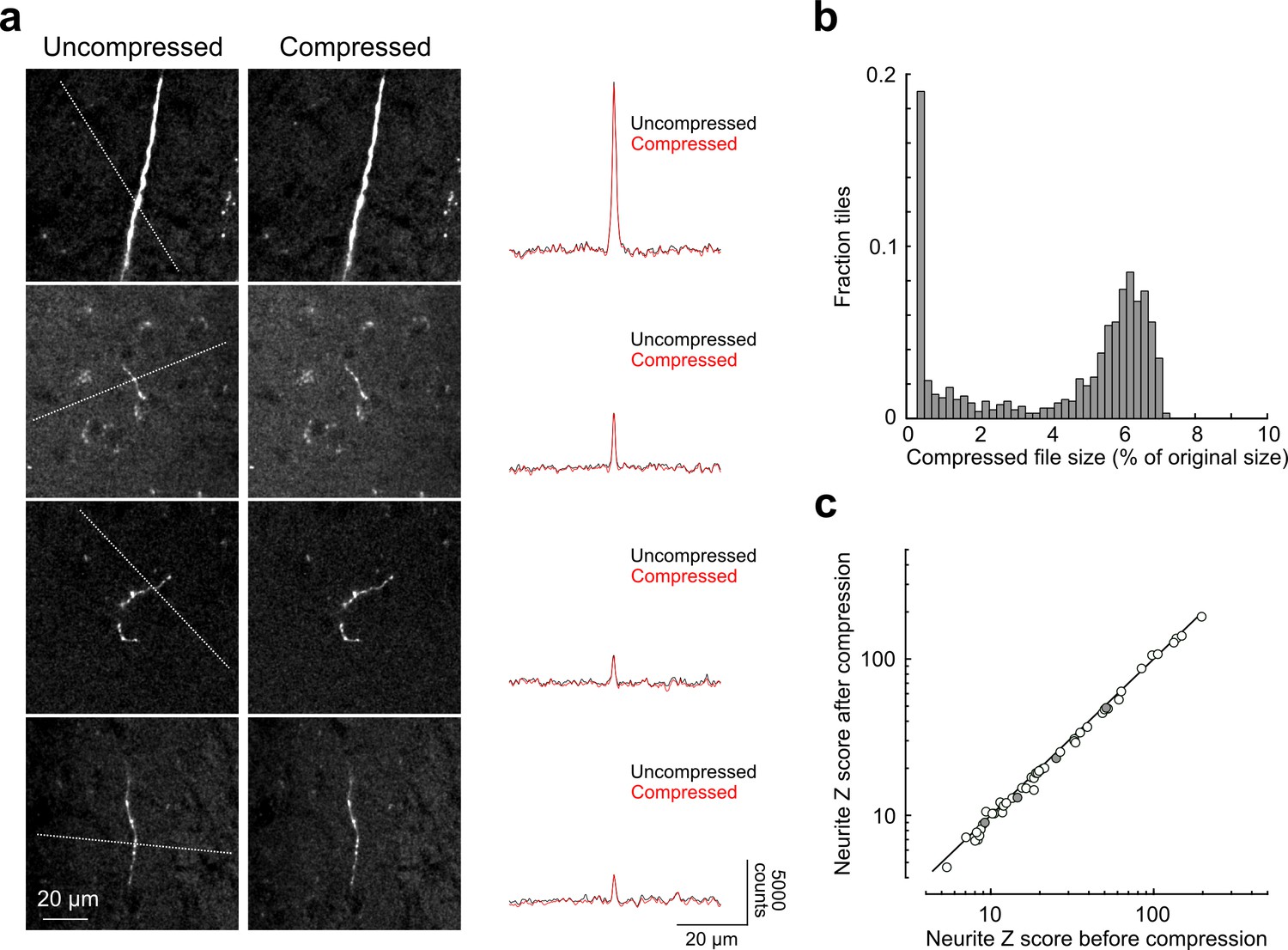
Signal-to-noise of axonal imaging.
(a) Representative images before (left) and after (middle) lossy H.264 compression. The intensity profile across each neurite (along paths denoted by dotted lines in images on left) is plotted to the right of each set of images and was minimally affected by image compression. (b) Distribution of compressed file size across a random sampling of 996 tiles. Across the entire subset, tiles were reduced in size by 95.7 ± 2.5% percent after compression. (c) SNR of axonal segments in each intensity profile (n = 52) before and after compression. SNR along each path was reduced to 95.12 ± 5.92% of control by the compression procedure. SNR, signal-to-noise ratio.
Figure 6
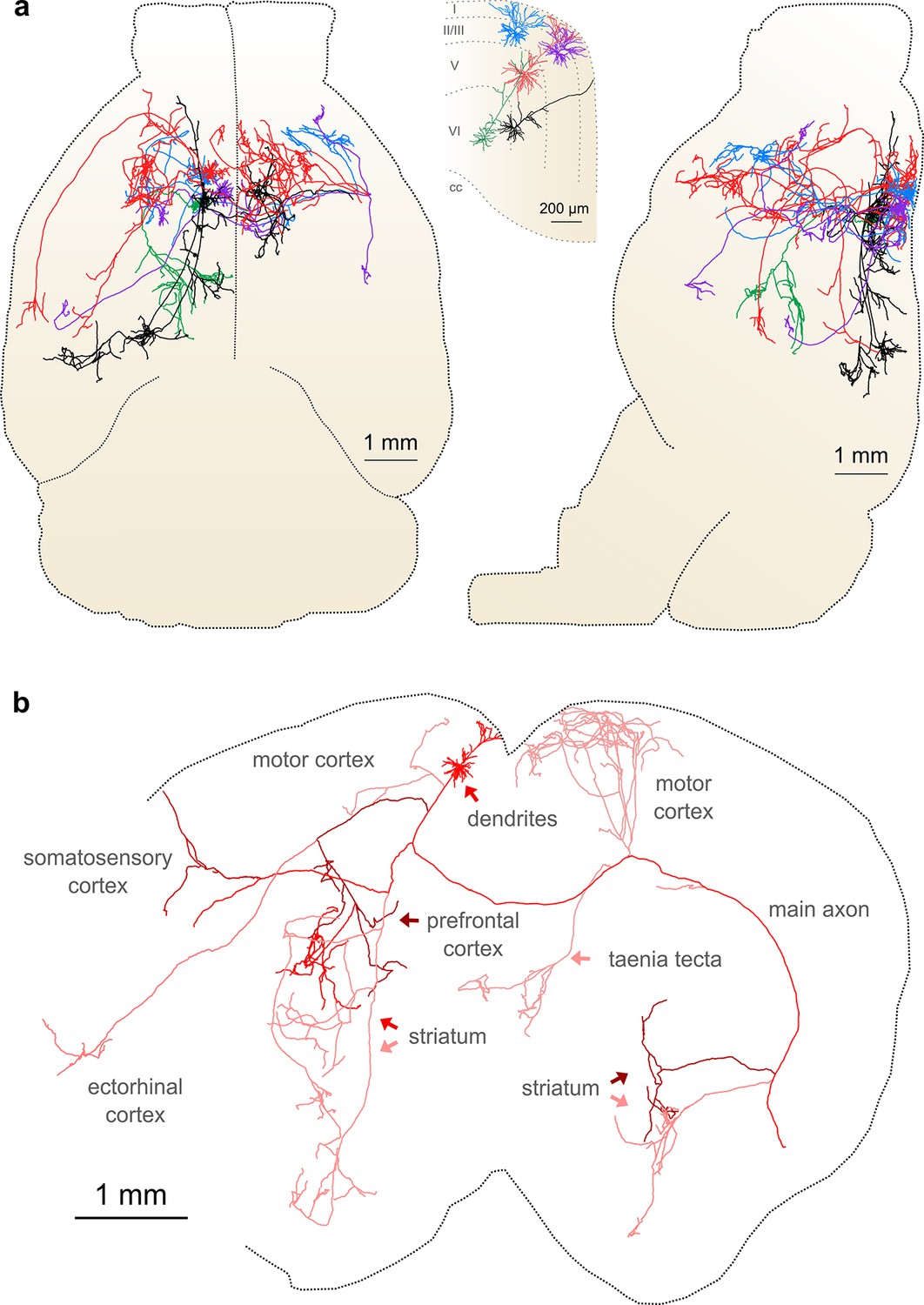
Complete reconstruction of axonal morphology.
(a) Complete reconstruction of the same five projection neurons depicted in Figure 4 (inset). Reconstructions are overlaid on a horizontal (left) and sagittal (right) outline of the imaged mouse brain. Subset includes pyramidal neurons in layer II (blue, purple), layer V (red, black) and layer VI (green). (b) Illustration of axonal and dendritic reconstruction of the layer 5 pyramidal cell (colored red in a) shown in the coronal plane. Profile of coronal section at the rostrocaudal position of the cell body is depicted by the black dashed line. Segments were colored to highlight axonal arbors originating from common branch points.
Figure 7
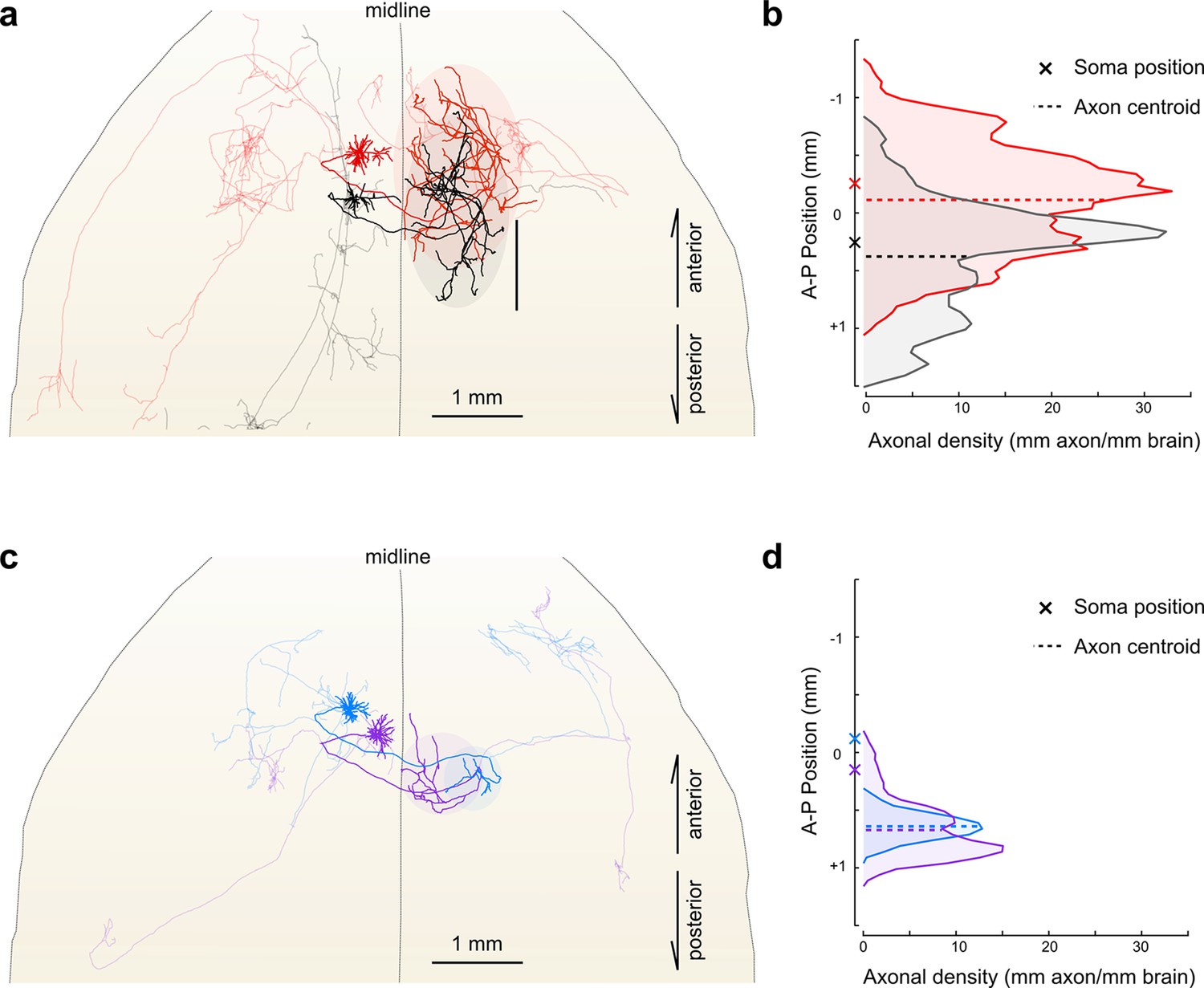
Fine scale topology of contralateral cortical projections.
(a) Horizontal view of the dendrites and axons of two layer V IT neurons (red and black). Axons projecting to locations other than the contralateral motor cortex are shown in lighter colors. (b) Density of axonal projections within the contralateral motor cortex as a function of position along the anterior–posterior (A–P) axis. Each point represents the cumulative length of axon within a 200 µm bin centered at the given coordinate divided by the bin width. A–P coordinates are relative to the center of the injection volume. (c) Horizontal view of Layer II IT neurons (blue and purple). Same view as in (a). (d) Density of axonal projections for the two neurons in (c) are on the same scale as in (b). Color codes are the same as in Figures 5 and 6.
Videos
Video 1
Movie illustrating 18 serially acquired image tiles that have been registered and resampled into a continuous image volume.
This volume (3 × 1 × 6 tiles) spans five adjacent tissue sections. Fine axons are resolvable and all fibers appear continuous. Images were spectrally unmixed to remove autofluorescence of lipofuscin.
Video 2
Single axon traced to its terminus.
Depicted path represents the longest continuous axonal segment starting at the cell soma. The terminus is located in the anterior piriform cortex. White dot corresponds to the same location in both panels and corresponds approximately to the path of manually traced segment. The SNR of well-labeled axons remains high along their entire length and branch points are clearly visible. Nuclei (magenta) were counter-labeled using NuclearID-Red. Two axons, originating from distinct neurons, cross in the corpus callosum. Axon identity is straightforward to assign in this example on the basis of trajectory and labeling intensity when viewed in three dimensions. This neuron appears blue in all figures.
Video 3
Three-dimensional rendering of reconstructed Layer II motor cortical neurons.
Displayed brain outline corresponds to the contours of the imaged brain. Color code is the same as in all figures.
Video 4
Three-dimensional rendering of reconstructed Layer V motor cortical neurons.
Displayed brain outline corresponds to the contours of the imaged brain. Color code is the same as in all figures.
Video 5
Three-dimensional rendering of reconstructed Layer VI motor cortical neuron.
Displayed brain outline corresponds to the contours of the imaged brain. Color code is the same as in all figures.
Tables
Table 1
Clearing solutions.
| Solution (#) | Dimethyl sulfoxide (g) | PB (g) | D-sorbitol (g) | Refractive index |
|---|---|---|---|---|
| 1 | 26.83 | 73.17 | 0.00 | 1.373 |
| 2 | 52.38 | 47.62 | 0.00 | 1.412 |
| 3 | 44.52 | 40.48 | 15.00 | 1.425 |
| 4 | 36.67 | 33.33 | 30.00 | 1.440 |
| 5 | 34.25 | 20.75 | 45.00 | 1.468 |
| 6 | 25.56 | 11.44 | 63.00 | 1.489 |
Table 2
Axonal reconstructions. All lengths in mm.
| Soma location | Layer II | Layer II | Layer V | Layer V | Layer VI |
|---|---|---|---|---|---|
| Dendritic branches | 66 | 57 | 37 | 25 | 23 |
| Dendritic length | 8.03 | 7.67 | 9.17 | 5.06 | 4.20 |
| Axonal branches | 79 | 67 | 178 | 136 | 27 |
| Axonal length | 47.34 | 41.04 | 121.20 | 75.44 | 23.57 |
| Axonal targets (ipsilateral) | Motor cortex Dorsal striatum Nucleus accumbens | Motor cortex Orbital cortex Dorsal/medial striatum Caudal/lateral striatum | Motor cortex Somatosensory cortex Auditory cortex Orbital cortex Agranular insular cortex Ectorhinal cortex Piriform cortex Dorsal striatum Nucleus accumbens Olfactory tubercle Taenia tecta | Motor cortex Somatosensory cortex Auditory cortex Anterior cingulate cortex Posterior parietal cortex | Motor cortex Thalamic nuclei: Ventral anterior lateral Posterior Submedial Reticular |
| Axonal targets (contralateral) | Motor cortex Insular cortex Piriform cortex | Motor cortex Anterior cingulate cortex Agranular insular cortex Claustrum Basolateral amygdala | Motor cortex Piriform cortex Dorsal striatum Nucleus accumbens Olfactory tubercle Taenia tecta | Motor cortex Anterior cingulate cortex Dorsal striatum |
Table 3
Comparison with alternative technologies for whole-brain imaging.
| Method | Lateral resolution (L; µm) | Axial resolution (A; µm) | L × L × A (µm3) | Speed (× 106 µm3/s) |
|---|---|---|---|---|
| This study | 0.45 | 1.33 | 0.26 | 1.6 |
| Selective plane illumination microscopy* | 0.65 | 7.30 | 3.10 | 160 |
| Knife-edge scanning microscopy/ micro-optical sectioning tomography (Li et al., 2010) | 0.71 | 1.0 | 0.50 | 1.0 |
| Transmission electron microscopy with camera array (Bock et al., 2011) | 0.004 | 0.045 | 7.2 x 10⁻⁷ | 5.6 x 10⁻⁶ |
| Serial block-face electron microscopy (Helmstaedter et al., 2013) | 0.0165 | >0.025 | >6.8 x 10⁻⁶ | 1.1 x 10⁻⁶ |
-
*Ideal resolution in fully cleared whole mouse brain (P. Keller, personal communication).
-
Comparison of resolution and imaging speed with other imaging modalities. Resolution values represent full width at half maximum except for in transmission electron microscopy with camera array and serial block-face electron microscopy, where pixel sizes are reported.
Download links
A two-part list of links to download the article, or parts of the article, in various formats.
Downloads (link to download the article as PDF)
Open citations (links to open the citations from this article in various online reference manager services)
Cite this article (links to download the citations from this article in formats compatible with various reference manager tools)
A platform for brain-wide imaging and reconstruction of individual neurons
eLife 5:e10566.
https://doi.org/10.7554/eLife.10566


