A computational pipeline to track chromatophores and analyze their dynamics
- Max Planck Institute for Brain Research, Germany
Figures
Figure 1
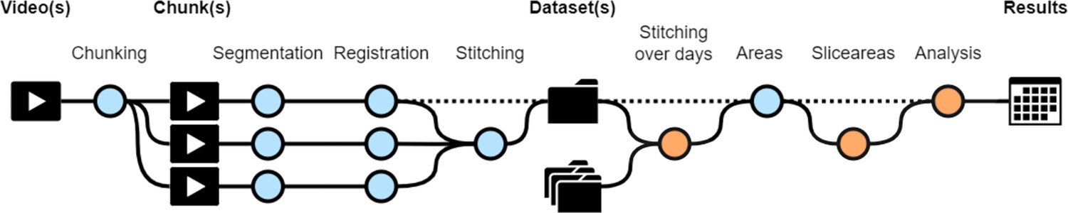
Workflow diagram of CHROMAS.
Dotted lines indicate optional steps in the process, allowing flexibility depending on experimental requirements. Orange dots represent new functions that did not exist in the initial versions of the pipeline (Reiter et al., 2018; Woo et al., 2023). Each step of the pipeline can be run independently, providing users with the flexibility to execute specific stages as needed. Additionally, CHROMAS includes options to generate visual output videos, enabling users to assess and validate the accuracy and quality of the result at every step.
Figure 2
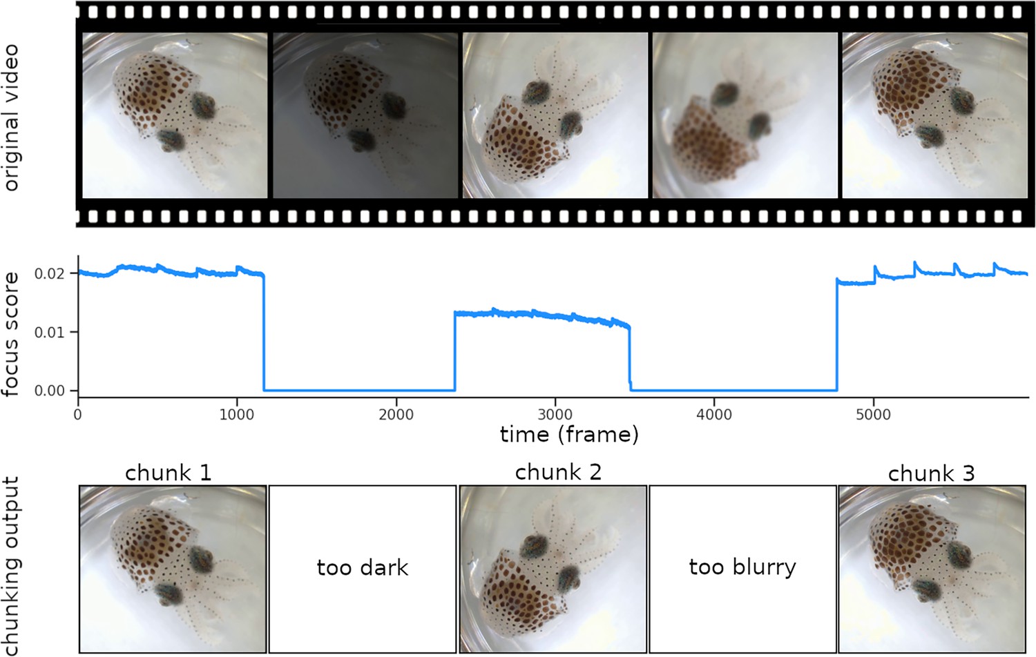
Chunking process.
The video frames are sorted based on their focus score. Images that are too dark or too blurry are removed from the dataset, and chunks made of consecutive sharp frames are created. In the figure above, the score decreases due to a brightness drop at frame 1200 and to the subject going out of focus around frame 3500, resulting in three distinct chunks. Continuity between chunks is reestablished during the ‘Stitching’ process (see Figure 5).
Figure 3
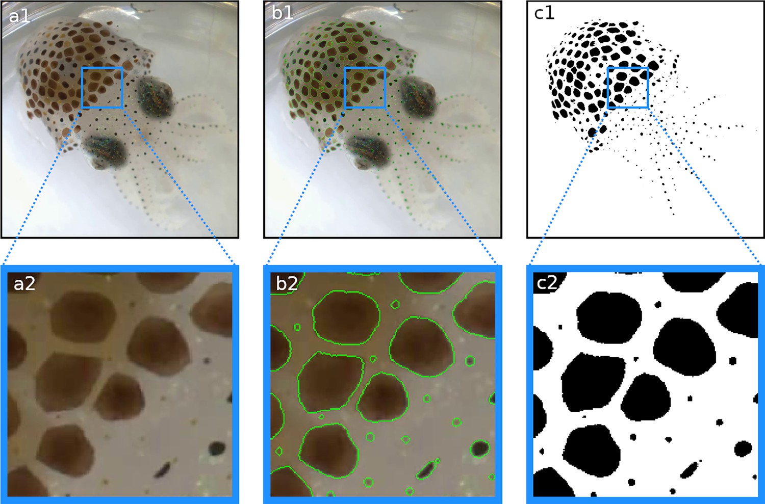
Segmentation results.
In each frame, each pixel is classified as either part of a chromatophore or not. (a1, a2) Original frame before segmentation. (b1, b2) Original frames with edges of segmented chromatophores in green. (c1, c2) Binary segmentation with chromatophores in black and background in white. Note that even the smallest chromatophores, though faint and difficult to discern on the original footage, are segmented.
Figure 4
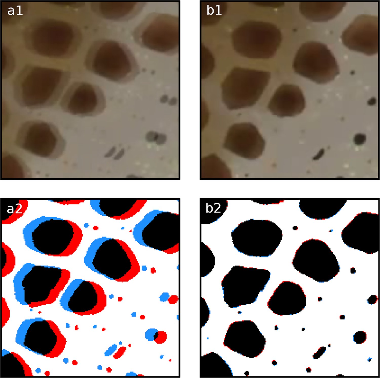
Registration.
Overlay of two frames 20 frames apart within the same chunk. Panels (a1, a2) illustrate the misalignment of two chromatophores (red and blue) before registration. Panels (b1, b2) show the same frames after automated registration. The registration process compensates for small movements or drifts over time, ensuring correct identification and tracking of the chromatophores over time.
Figure 5
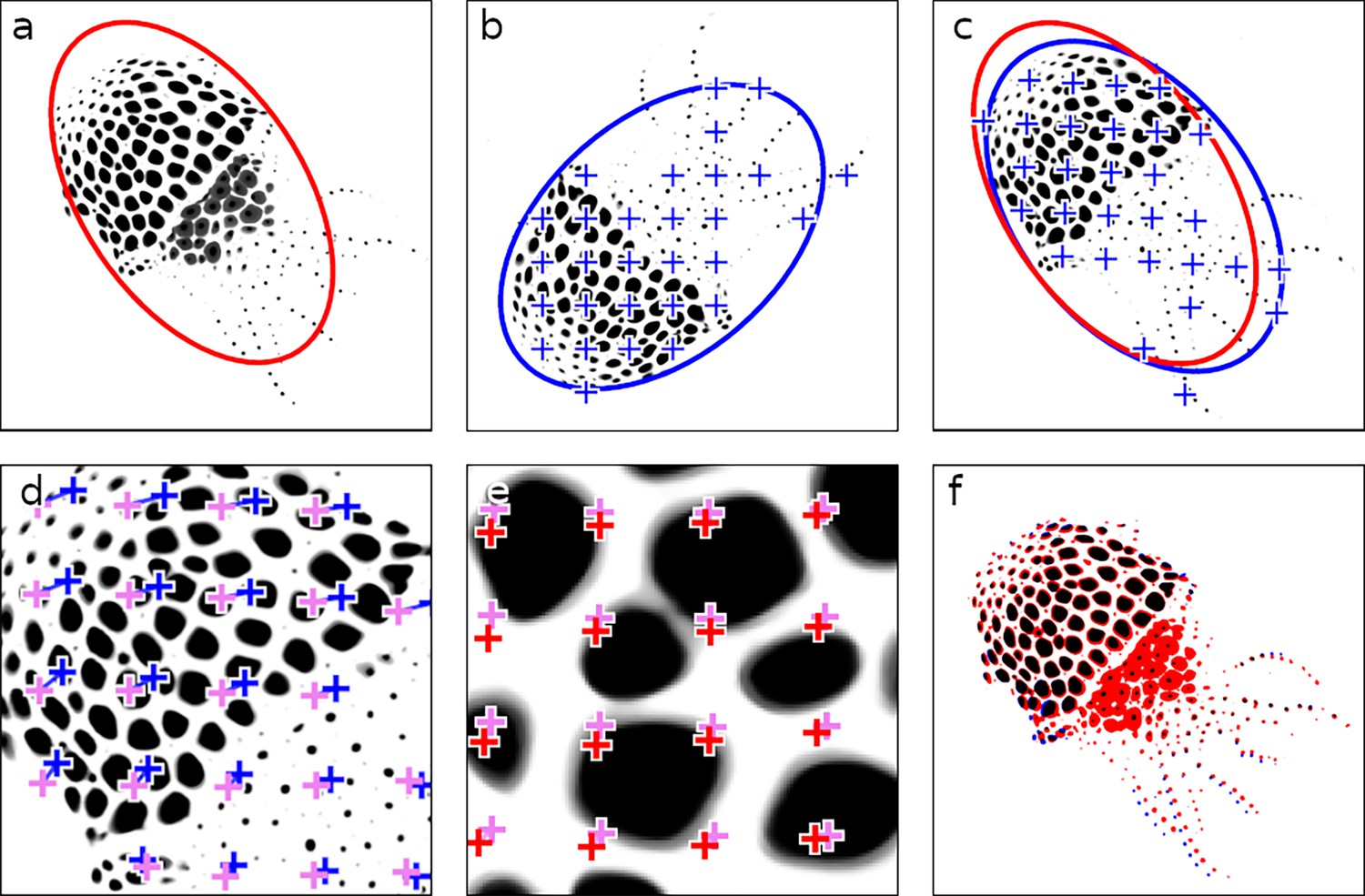
Stitching video chunks.
This figure illustrates the stepwise refinement process for stitching adjacent video chunks, ensuring precise alignment critical for downstream analyses. (a) Masterframe of chunk 1, with an initial ellipse fit shown in red. (b) Masterframe of chunk 2, featuring the ellipse fit and a grid of points for fine alignment in blue. (c) Chunk 2 aligned on chunk 1 using the ellipse-fitting method. (d) First round of fine alignment, maximizing phase correlation between patches surrounding the points. Points prior to fine alignment are shown in blue, and their adjusted positions post-alignment are in pink. (e) Second round of fine alignment, from pink to red. (f) Final overlay between chunk 1 and the fully aligned chunk 2. In black are the chromatophore areas common to both chunks; in red and blue are chromatophore areas that are unique to chunks 1 and 2, respectively.
Figure 6
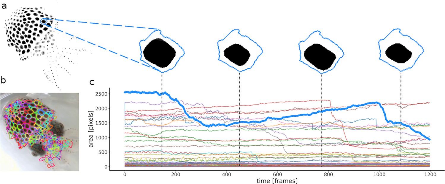
Calculation of chromatophore areas.
(a) Masterframe and zoom on the segmentation of one chromatophore’s contractions and expansions. (b) Cleanqueen. Each color represents a different chromatophore territory. (c) Surface area of each segmented chromatophore over time (colors as in b). The chromatophore in a is highlighted in the thick blue line. This approach measures the total area occupied by a chromatophore within its defined territory and offers no information about its shape.
Figure 7
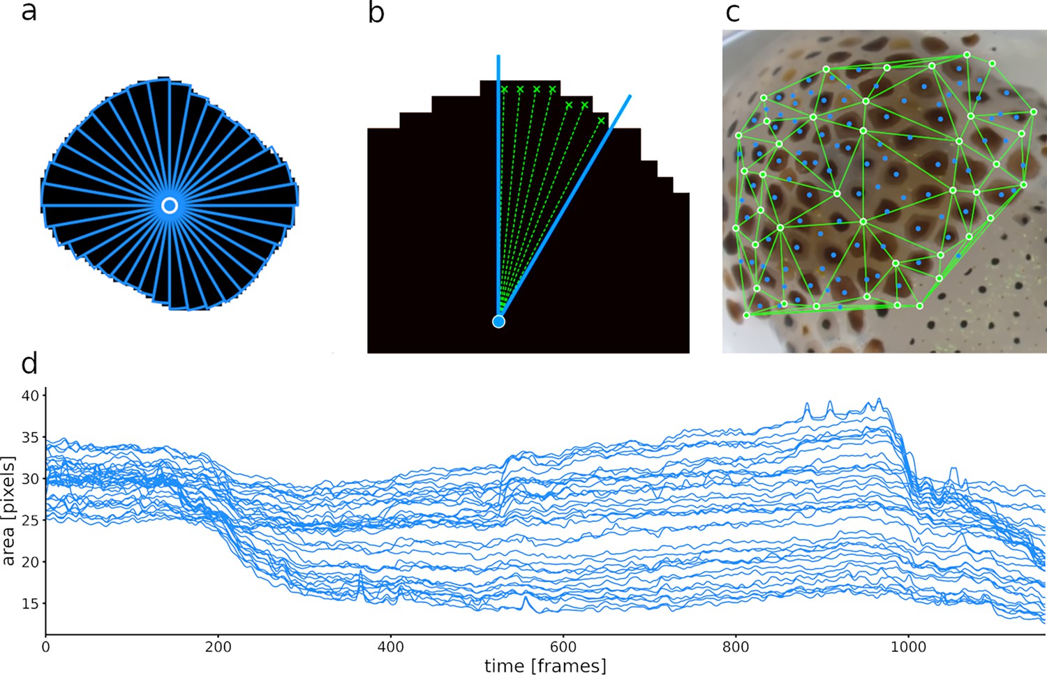
Calculation of slice surface areas.
(a) A single chromatophore (the same one as in Figure 6) is divided radially into 36 slices. (b) Close-up on one of the 36 slices, indicating how its surface area is estimated. (c) Chromatophore ‘epicenters’ (see text) in blue and motion markers (see text) in green, with edges for triangulation. (d) Plot representing the surface areas of the 36 slices of this chromatophore over time. Note that the dynamics of a chromatophore are now described by 36 values per frame, rather than one, as in Figure 6c. Note also that the top half of the traces describing this chromatophore deviates clearly from the others around frames 550 and 960, indicating their differential control. This fine-grain description of chromatophore deformations over time is used to reveal the fine details of their individual and collective motor control.
Figure 8
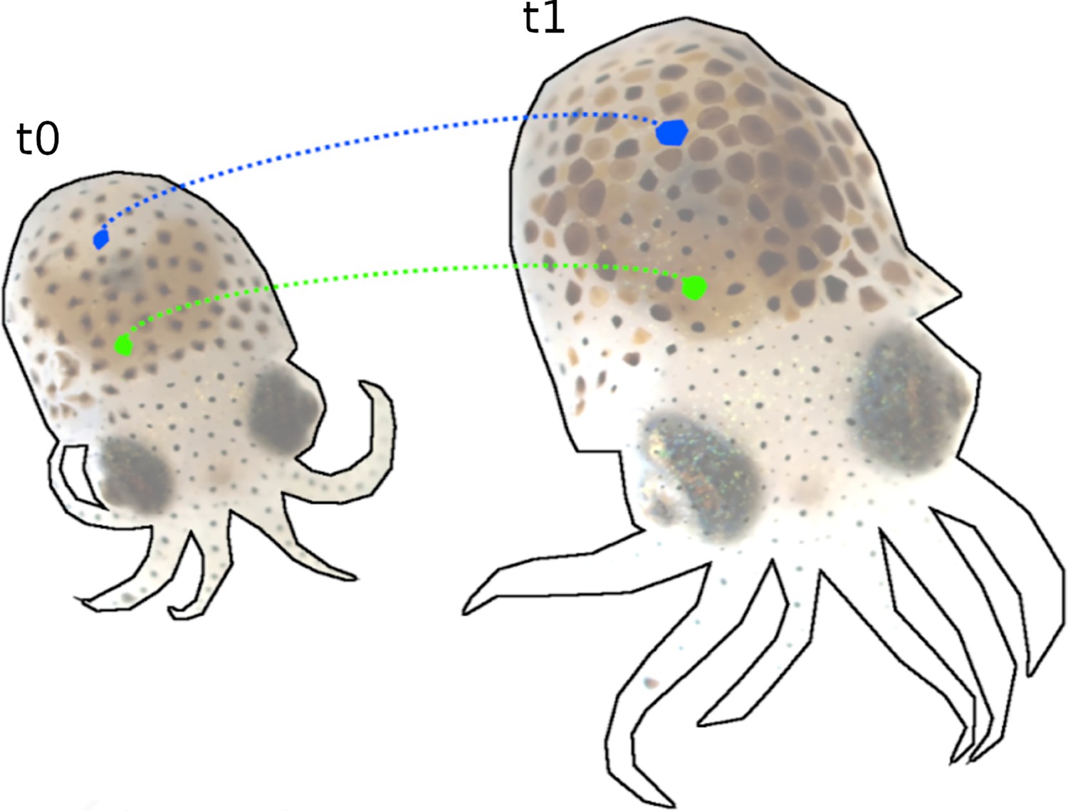
Tracking of chromatophores over 12 days of development (t0 = 7 days post hatching (dph) and t1 = 21 dph).
During this time, the number of chromatophores nearly doubled, with many changing chromatic properties. Despite these changes and intermittent filming, our pipeline reliably tracks individual chromatophores, as illustrated with two arbitrarily selected chromatophores, in blue and green.
Figure 9
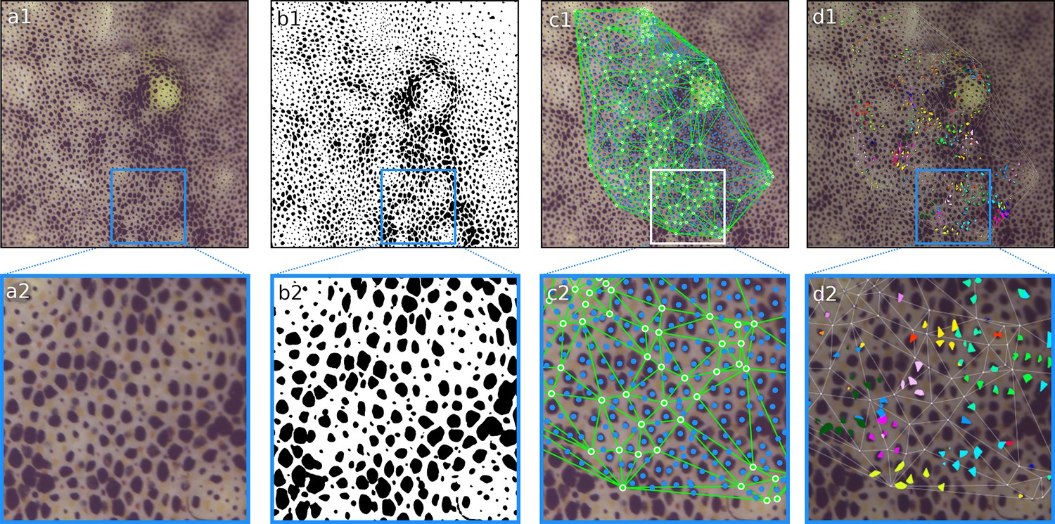
Example of 4K footage of Sepia officinalis processed through the CHROMAS pipeline.
(a1, a2) Original video frame. (b1, b2) Binary segmentation with chromatophores in black and background in white. (c1, c2) Epicenters of chromatophores in blue and motion markers with triangulation in green. (d1, d2) Putative motor units calculated using the Affinity Propagation algorithm. In this example, Principal Component Analysis–Independent Component Analysis (PCA–ICA) revealed independent components influencing the activity of each chromatophore. We found 4.68 ± 1.41 (mean ± std) ICs per chromatophore (n = 1616). Those independent components were then clustered together based on their covariation and plotted with the same color. For visualization purposes, only clusters of size 8 and 9 are plotted. In this segment, we found 10.37 ± 14.23 (mean ± std) chromatophores per cluster, with 90% of clusters consisting of less than 20 chromatophores. This example highlights CHROMAS’s ability to process complex datasets, such as footage of Sepia officinalis, which exhibits a high density of chromatophores and very active dynamics correlated with its camouflage and other behaviors.
Tables
Table 1
Performance on a workstation with a 10-core Intel Core i9-10900X with 64 GB RAM and a NVIDIA RTX A4000 GPU.
Runtime in milliseconds per frame (mean ± s.d.).
| Resolution | Number of chromatophores (ms/frame) | Segmentation(neural net) (ms/frame) | Registration (ms/frame) | Tracking chromatophore size (ms/frame) | Tracking anisotropic activity (ms/frame) |
|---|---|---|---|---|---|
| SD | 146 | 5.38 ± 0.1 | 18.61 ± 0.1 | 13.01 ± 1.4 | 4.98 ± 0.9 |
| HD | 566 | 22.31 ± 0.7 | 62.87 ± 2.3 | 140.44 ± 1.0 | 135.24 ± 0.9 |
| k | 2842 | 986.21 ± 10.4 | 611.74 ± 5.4 | 744.69 ± 2.5 | 495.17 ± 2.8 |
Table 2
Performance on a laptop with a 4-core Intel Core i5-1135G7 with 16 GB RAM and no NVIDIA GPU.
Runtime in milliseconds per frame (mean ± s.d.).
| Resolution | Number of chromatophores (ms/frame) | Segmentation(lookup) (ms/frame) | Registration (ms/frame) | Tracking chromatophore size (ms/frame) | Tracking anisotropic activity (ms/frame) |
|---|---|---|---|---|---|
| SD | 146 | 11.55 ± 1.81 | 4.67 ± 0.63 | 14.56 ± 5.1 | 9.31 ± 0.6 |
| 4k | 2842 | 1679.62 ± 251.8 | 1490.94 ± 249.9 | 3072.94 ± 121.6 | 1488.25 ± 84.0 |
Appendix 1—key resources table
| Reagent type (species) or resource | Designation | Source or reference | Identifiers | Additional information |
|---|---|---|---|---|
| Strain, strain background | Euprymna berryi (bobtail squid) | Laurent Lab, Max Planck Institute for Brain Research | Lab-reared; used in developmental tracking and anisotropy analysis | |
| Strain, strain background | Sepia officinalis (European cuttlefish) | Laurent Lab, Max Planck Institute for Brain Research | Used for high-density chromatophore datasets | |
| Software, algorithm | CHROMAS | This paper; https://doi.org/10.17617/1.pa38-mh49 | Pipeline for chromatophore segmentation and analysis | |
| Software, algorithm | Python | Python Software Foundation; https://www.python.org/ | Version 3.9+ | |
| Software, algorithm | PyTorch | Paszke et al., 2019; https://pytorch.org/ | For segmentation models | |
| Software, algorithm | Torchvision | Marcel and Rodriguez, 2010; https://pytorch.org/vision/ | Model architectures | |
| Software, algorithm | OpenCV | Bradski, 2000; https://opencv.org/ | Image and video processing | |
| Software, algorithm | scikit-learn (1.6.1) | Pedregosa et al., 2011; https://scikit-learn.org/ | Clustering and dimensionality reduction | |
| Software, algorithm | scikit-image (0.24.0) | van der Walt et al., 2014; https://scikit-image.org/ | Image processing | |
| Software, algorithm | albumentations (1.4.24) | Buslaev et al., 2020; https://albumentations.ai/ | Data augmentation | |
| Software, algorithm | xarray (2024.11.0) | Hoyer and Hamman, 2017; http://xarray.pydata.org/ | Labeled multi-dimensional arrays | |
| Software, algorithm | Zarr (2.18.4) | Miles et al., 2020; https://zarr.readthedocs.io/ | Chunked data storage | |
| Software, algorithm | Dask (2024.12.1) | Dask Development Team, 2016; https://www.dask.org/ | Parallel and distributed processing | |
| Software, algorithm | decord | Wang, 2019; https://github.com/dmlc/decord | Efficient video loading | |
| Software, algorithm | Matplotlib (3.10.0) | Hunter, 2007; https://matplotlib.org/ | Visualization | |
| Software, algorithm | Bokeh (3.6.2) | Bokeh Development Team, 2014; https://bokeh.org/ | Interactive dashboards | |
| Software, algorithm | Click (8.1.8) | Ronacher, 2014; https://click.palletsprojects.com/ | CLI for CHROMAS | |
| Software, algorithm | tqdm (4.67.1) | tqdm Developers, 2016; https://github.com/tqdm/tqdm | Progress bars | |
| Software, algorithm | Trogon (0.3.0) | Freeman, 2022; https://github.com/Textualize/trogon | Terminal GUI | |
| Software, algorithm | Sphinx | Sphinx Team, 2007; https://www.sphinx-doc.org/ | Documentation generation | |
| Software, algorithm | nbsphinx (0.9.6) | Grünwald, 2017; https://github.com/spatialaudio/nbsphinx | Integrates Jupyter notebooks in Sphinx | |
| Software, algorithm | jupyter-client | Jupyter Development Team, 2015; https://jupyter.org/ | Jupyter support | |
| Software, algorithm | Pandoc (2.4) | MacFarlane, 2006; https://pandoc.org/ | Document conversion | |
| Software, algorithm | rpy2 | Gautier, 2008; https://github.com/rpy2/rpy | R–Python bridge | |
| Other | Pre-trained chromatophore segmentation models | This paper; https://public.brain.mpg.de/Laurent/Chromas2025/ | Trained on *E. berryi* and *S. officinalis* | |
| Other | Workstation (Intel i9-10900X+RTX A4000) | Laurent Lab, Max Planck Institute for Brain Research | Used for performance benchmarking | |
| Other | Laptop (Intel i5-1135G7, no GPU) | Laurent Lab, Max Planck Institute for Brain Research | Used to demonstrate pipeline performance on CPU |
Additional files
Download links
A two-part list of links to download the article, or parts of the article, in various formats.
Downloads (link to download the article as PDF)
Open citations (links to open the citations from this article in various online reference manager services)
Cite this article (links to download the citations from this article in formats compatible with various reference manager tools)
A computational pipeline to track chromatophores and analyze their dynamics
eLife 14:RP106509.
https://doi.org/10.7554/eLife.106509.3


