Figures and data in Domain coupling in allosteric regulation of SthK measured using time-resolved transition metal ion FRET

Figures
Tables
Additional files

8 figures, 2 tables and 1 additional file

Figures

Figure 1

Download asset Open asset

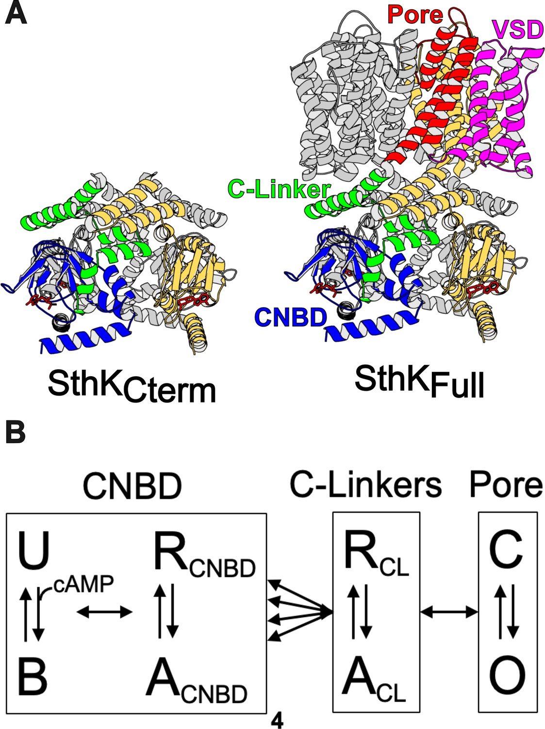
Structure of SthK constructs and modular gating scheme.

(A) Cartoon structures for SthK_Cterm and SthK_Full with the domains labeled on the SthK_Full structure. (B) Modular gating scheme for SthK showing modules corresponding to domains indicated in the structures above. Within each domain, resting (R) and active (A) or closed (C) and open (O) or unbound (U) and bound (B) conformations are shown connected by double arrows, representing the transition between states. Horizontal arrows between modules indicate the coupling between domains.

Figure 2

Download asset Open asset

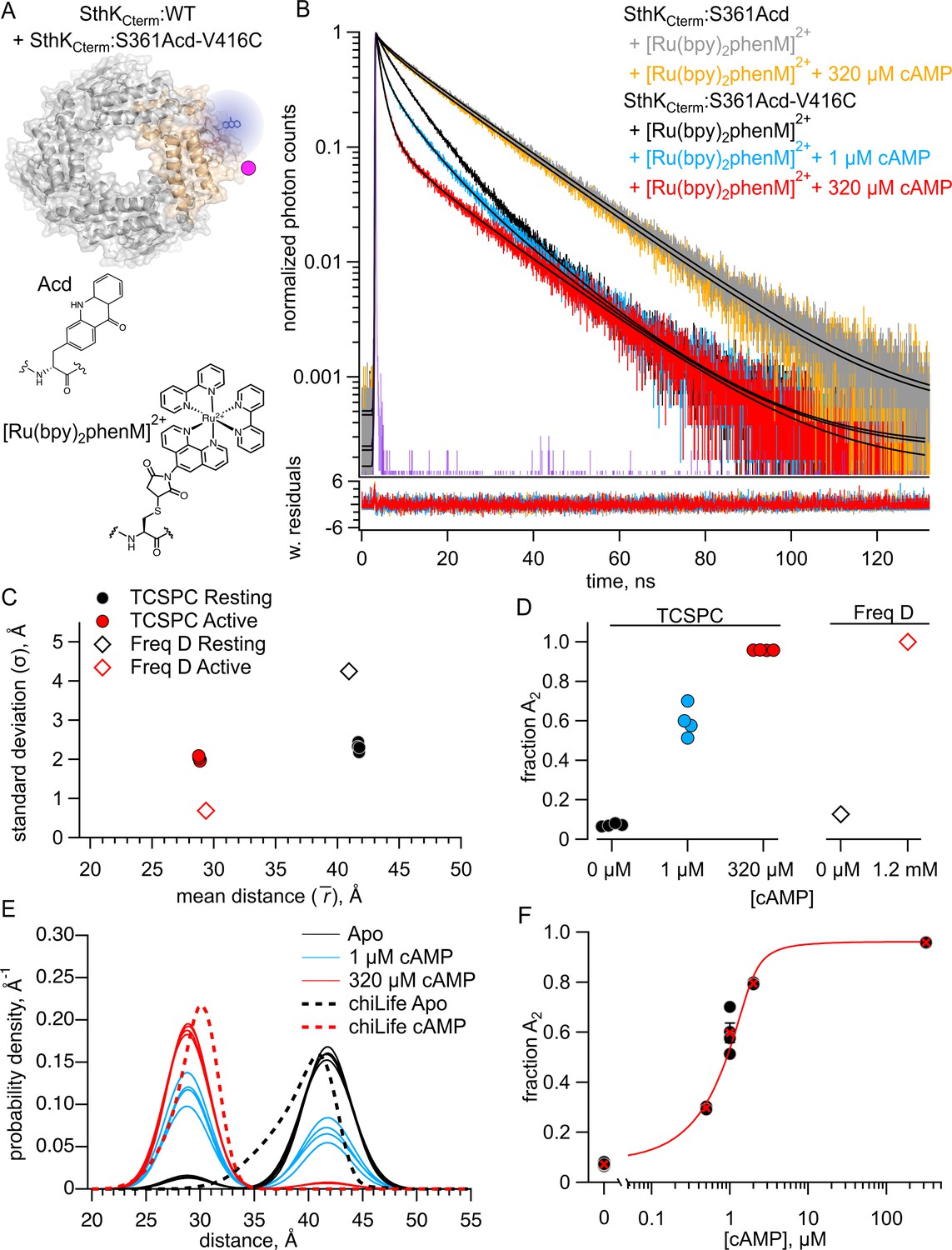
Förster resonance energy transfer (FRET) with the donor-acceptor pair within the same subunit.

(A) Cartoon of SthK_Cterm:WT/S361Acd-V416C with a single donor-acceptor labeled subunit (top; acceptor shown as magenta dot) and the structures of donor fluorophore, Acd, and acceptor metal complex [Ru(bpy)₂phenM]²⁺ (bottom). (B) Representative TCSPC data from SthK_Cterm:WT/S361Acd treated with [Ru(bpy)₂phenM]²⁺ before (gray) and after (orange) the addition of 320 μM cAMP. Time-correlated single photon counting (TCSPC) data from SthK_Cterm:WT/S361Acd-V416C treated with [Ru(bpy)₂phenM]²⁺ in the absence of cAMP (black) and in the presence of 1 μM (blue) or 320 μM (red) cAMP. Smooth black curves show the fits of the FRET model, and weighted residuals are shown below using the same colors as used for the data. Representative instrument response function (IRF) shown in purple. (C) Summary of distance parameter values, $\bar{r}$ and $σ$ (n=4), from fits to our TCSPC data (filled symbols) and from previously published frequency domain data (open symbols), with resting and active state as indicated in the legend (Eggan et al., 2024). (D) $f_{A 2}$ values determine from fits to TCSPC data measured with 0, 1 μM and 320 μM cAMP (filled symbols) compared to previously published $f_{A 2}$ values determine from frequency domain data (open symbols) (Eggan et al., 2024). (E) Spaghetti plot of distance distributions from individual experiments for 0 (black), 1 μM (blue) and 230 μM (red) cAMP, with distributions predicted by chiLife shown as dashed curves. Resting and active are shown in black and red, respectively. (F) Summary of $f_{A 2}$ values over a range of cAMP concentrations. The dose-response relation was fit with a quadratic equation (red curve) with *K_D* = 0.22 μM and ${[P]}_{t o t a l}$ = 1.2 μM.

Figure 2—source data 1 Excel data for time-correlated single photon counting (TCSPC) representative traces, dot plot, scatter plot, spaghetti plot, and dose response plot from Förster resonance energy transfer (FRET) experiments within SthK_Cterm subunits (Figure 2B–F).: https://cdn.elifesciences.org/articles/106892/elife-106892-fig2-data1-v1.xlsx
Download elife-106892-fig2-data1-v1.xlsx

Figure 3

Download asset Open asset

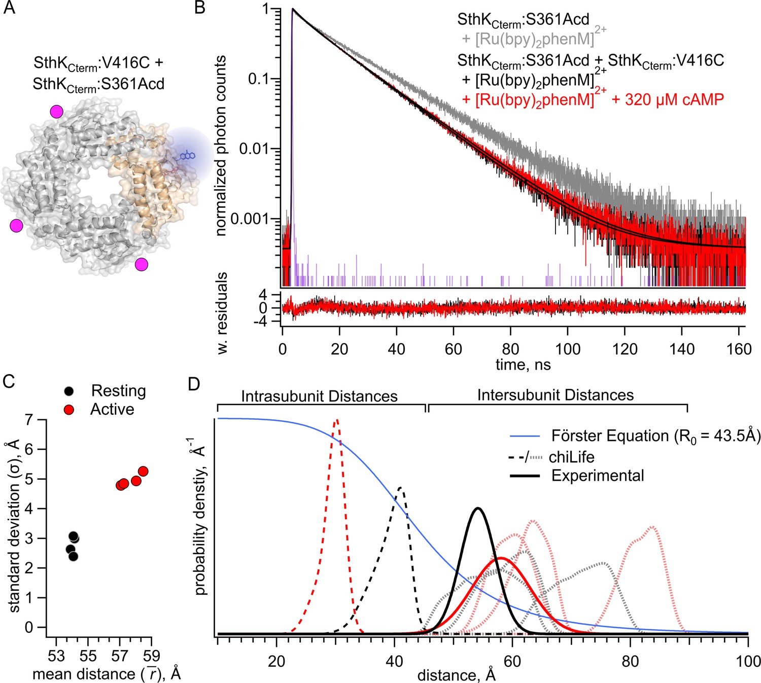
Förster resonance energy transfer (FRET) with the donor-acceptor pair on different subunits.

(A) Cartoon structure of SthK_Cterm:V416C/S361Acd protein with a single donor-labeled subunit (SthK_Cterm:S361Acd) and three acceptor-labeled subunits (SthK_Cterm:V416C). (B) Representative TCSPC data from the donor-only condition (gray), and after [Ru(bpy)₂phenM]²⁺ labeling either in the absence (black) or presence (red) of 320 μM cAMP, fit with the FRET model (smooth black lines). The instrument response function (IRF) and weighted residuals are depicted as in Figure 2. (C) Summary of distance parameter values, $\bar{r}$ and $σ$ (n=4), from fits of our time-correlated single photon counting (TCSPC) data with the FRET model. Resting and active states are shown as black and red, respectively. (D) Distributions of donor-acceptor distances predicted with chiLife for intrasubunit distances (darker dashed curves) and intersubunit distances (lighter dashed curves), with black and red as described in (C). The distance distributions from fits to our TCSPC data for resting and active states are overlaid as solid black and red Gaussians.

Figure 3—source data 1 Excel data for time-correlated single photon counting (TCSPC) representative traces, dot plot, and spaghetti plot from Förster resonance energy transfer (FRET) experiments between SthK_Cterm subunits (Figure 3B–D).: https://cdn.elifesciences.org/articles/106892/elife-106892-fig3-data1-v1.xlsx
Download elife-106892-fig3-data1-v1.xlsx

Figure 4

Download asset Open asset

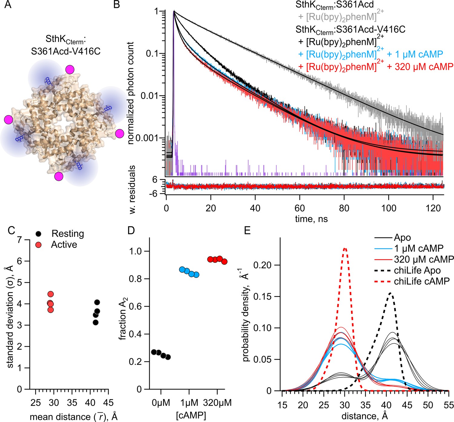
Förster resonance energy transfer (FRET) with both intrasubunit and intersubunit donor-acceptor pairs in SthK_Cterm.

(A) Cartoon structure of homotetrameric SthK_Cterm:S361Acd-V416C protein. (B) Representative time-correlated single photon counting (TCSPC) data from the donor-only condition (in gray) and after [Ru(Bpy)₂phenM]²⁺ labeling in the absence of cAMP (black) and in the presence of either 1 μM (blue) or 320 μM (red) cAMP, fit with the FRET model (smooth black lines). The instrument response function (IRF) and weighted residuals are depicted as in Figure 2. (C) Summary of distance parameter values, $\bar{r}$ and $σ$ (n=4), from fits of our TCSPC data with the FRET model. Resting and active states are shown as black and red, respectively. (D) Values of $f_{A 2}$ for 0, 1 μM or 320 μM cAMP, as indicated. (E) Spaghetti plot of distance distributions from individual experiments for 0 (black), 1 μM (blue) and 230 μM (red) cAMP, with distributions predicted by chiLife shown as dashed curves. Resting and active are indicated by black and red, respectively.

Figure 4—source data 1 Excel data for time-correlated single photon counting (TCSPC) representative traces, dot plot, scatter plot, and spaghetti plot from experiments with SthK_Cterm and inter- and intra-subunit Förster resonance energy transfer (FRET) (Figure 4B–E).: https://cdn.elifesciences.org/articles/106892/elife-106892-fig4-data1-v1.xlsx
Download elife-106892-fig4-data1-v1.xlsx

Figure 5

Download asset Open asset

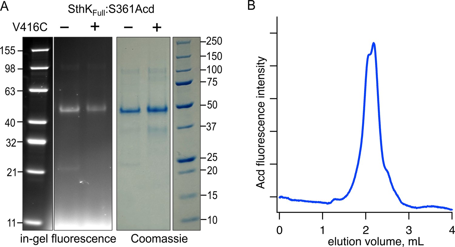
Expression and purification of SthK_Full incorporating Acd.

(A) SDS/PAGE with in-gel fluorescence (left) or Coomassie blue (right) for SthK_Cterm:S361Acd and SthK_Cterm:S361Acd-V416C, as indicated (theoretical mass = 53.0 kDa). (B) Chromatogram from size exclusion chromatography monitoring fluorescence at 425 nm (Acd) for SthK_Cterm:S361Acd-V416C.

Figure 5—source data 1 Original uncropped in-gel fluorescence and Coomassie protein gel image (Figure 5A).: https://cdn.elifesciences.org/articles/106892/elife-106892-fig5-data1-v1.zip
Download elife-106892-fig5-data1-v1.zip
Figure 5—source data 2 Original labeled in-gel fluorescence and Coomassie protein gels for SthK_Full protein (Figure 5A).: https://cdn.elifesciences.org/articles/106892/elife-106892-fig5-data2-v1.zip
Download elife-106892-fig5-data2-v1.zip
Figure 5—source data 3 Excel data for size exclusion chromatography (Figure 5B).: https://cdn.elifesciences.org/articles/106892/elife-106892-fig5-data3-v1.xlsx
Download elife-106892-fig5-data3-v1.xlsx

Figure 6

Download asset Open asset

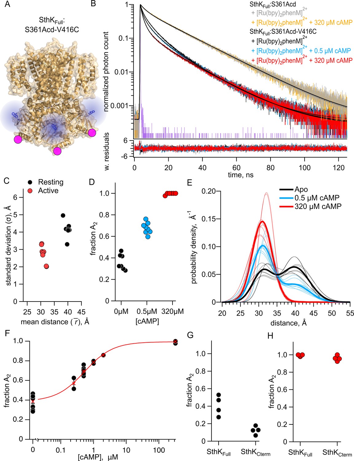
Förster resonance energy transfer (FRET) with both intrasubunit and intersubunit donor-acceptor pairs in SthK_Full.

(A) Cartoon structure of SthK_Full:S361Acd-V416C construct. (B) Representative time-correlated single photon counting (TCSPC) data from the donor-only condition (no cAMP – gray, 320 µM cAMP – orange) and SthK_Full:S361Acd-V416C after [Ru(bpy)₂phenM]²⁺ labeling in the absence of cAMP (black) and in the presence of either 1 μM (blue) or 320 μM (red) cAMP, fit with the FRET model (smooth black lines). The instrument response function (IRF) and weighted residuals are depicted as in Figure 2. (C) Summary of distance parameter values, $\bar{r}$ and $σ$ (n=4), from fits of our TCSPC data with the FRET model. Resting and active states are shown as black and red, respectively. (D) Values of $f_{A 2}$ for 0, 1 μM or 320 μM cAMP, as indicated. (E) Spaghetti plot of distance distributions from individual experiments for 0 (black), 1 μM (blue) and 230 μM (red) cAMP, with distributions predicted by chiLife shown as dashed curves. Resting and active are indicated by black and red, respectively. (F) Summary of $f_{A 2}$ over range of cAMP concentrations. The dose-response relation was fit with a quadratic equation (red curve) with *K_D* = 0.53 μM and ${[P]}_{t o t a l}$ = 0.025 μM. (**G–H**) Values of $f_{A 2}$ from globally fitting SthK_Full and SthK_Cterm constructs.

Figure 6—source data 1 Excel data for time-correlated single photon counting (TCSPC) representative traces, scatter plot, spaghetti plot, dose response plot, and dot plots from experiments with SthK_Full (Figure 2B–H).: https://cdn.elifesciences.org/articles/106892/elife-106892-fig6-data1-v1.xlsx
Download elife-106892-fig6-data1-v1.xlsx

Figure 7

Download asset Open asset

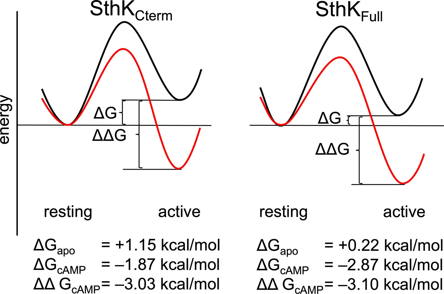
Energetics of the resting to active conformational change in the cyclic nucleotide-binding domain (CNBD).

A hypothetical reaction coordinate shows the relative energy difference between resting and active states (ΔG) and difference in free energy change (ΔΔG) without ligand (black) and with cAMP bound (red), for SthK_Cterm (left) and SthK_Full (right). Calculated ΔG and ΔΔGs values are shown for each construct below the diagram.

Figure 8 with 2 supplements

Download asset Open asset

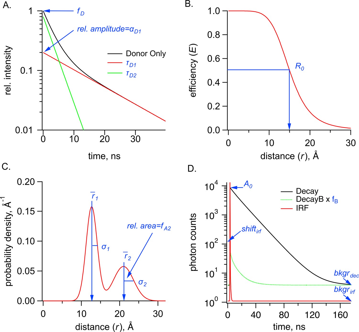
Parameters used in the Förster resonance energy transfer (FRET) model, shown in blue, for time-correlated single photon counting (TCSPC) data for the sum of two Gaussian distributions.

(A) Graph of donor-only fluorescence-lifetime decay with two exponential components with time constants ( $τ_{D 1}$ , $τ_{D 2}$ ). The amplitude fraction of the donor-only lifetime in an experiment is determined as $f_{D}$ . (B) FRET efficiency (E) plot as a function of distance (r) between donor and acceptor and the R₀ values for 50% FRET transfer. (C) Probability distribution plot of donor and acceptor distances P(r) showing the sum of two Gaussian distributions, each with their own average distance ( $\bar{r_{1}}$ and $\bar{r_{2}}$ ), standard deviations ( $σ_{1}$ and $σ_{2}$ ) and relative amplitude of the second component ( $f_{A 2}$ ). (D) Example TCSPC data is shown with experimental measured photon count data (Decay), the instrument response function (IRF), and the buffer only decay (DecayB), with its corresponding scaling factor $f_{B}$ relative to the Decay trace. Also indicated is a time-independent background of photon counts for the Decay trace, ${b k g r}_{d e c}$ , as well as two parameters associated with the IRF, its background, ${b k g r}_{i r f}$ , and the shift between instrument response function and measured decay, ${s h i f t}_{i r f}$ . Parameter $A_{0}$ is the amplitude of the FRET model estimate of the fluorescence lifetime of the donor (in photon counts).

Figure 8—figure supplement 1

Download asset Open asset

Identifiability of Individual Model Parameters.

(A) Identifiability of parameters in the sum of two Gaussian distributions model for representative time-correlated single photon counting (TCSPC) data. (A) Dependence of the reduced $χ^{2}$ values on the fraction of donor-only component ( $f_{D}$ ). (**B–C**) Dependence of the reduced $χ^{2}$ values on the Gaussian average distances ( $\bar{r}$ ) (B) and standard deviations ( $σ$ ) (C) for the resting (black) and active states (red). (D) Dependence of the reduced $χ^{2}$ values on the parameter $f_{A 2}$ for the conditions of apo, 0.5 μM, 1 μM and 320 μM cAMP.

Figure 8—figure supplement 1—source data 1 Excel data of χ² minimized curves across various parameters (Figure 8—figure supplement 1).: https://cdn.elifesciences.org/articles/106892/elife-106892-fig8-figsupp1-data1-v1.xlsx
Download elife-106892-fig8-figsupp1-data1-v1.xlsx

Figure 8—figure supplement 2

Download asset Open asset

Correlation Between Model Parameters.

(**A–F**) Parameter correlations for representative time-correlated single photon counting (TCSPC) data of $χ^{2}$ values in three dimensions.

Plots of $χ^{2}$ values vs. $σ_{1}$ and $f_{D}$ (A), vs. $σ_{2}$ and $f_{D}$ (B), vs. $f_{A 2}$ in 0 μM cAMP and $f_{D}$ (C), vs. $f_{A 2}$ in 320 μM cAMP and $f_{D}$ (D), vs $σ_{1}$ and ${\bar{r}}_{1}$ (E) and vs. $σ_{2}$ and ${\bar{r}}_{1}$ (F).

Figure 8—figure supplement 2—source data 1 Excel data of χ² minimized surfaces between various parameters (Figure 8—figure supplement 2).: https://cdn.elifesciences.org/articles/106892/elife-106892-fig8-figsupp2-data1-v1.xlsx
Download elife-106892-fig8-figsupp2-data1-v1.xlsx

Tables

Key resources table

Reagent type (species) or resource	Designation	Source or reference	Identifiers	Additional information
Strain, strain background (Escherichia coli)	B-95.ΔA E. coli	Addgene	Bacterial strain #197933	Electrocompetent cells
Recombinant DNA reagent	pDule2-Mj Acd A9 (plasmid)	Addgene	Plasmid #197652	Provided by GCE4Alls
Software, algorithm	TDlifetime_20_Igor_procedures.ipf	This paper	https://github.com/zagotta/TDlifetime_program	Code used for analyzing TCSPC lifetime data for use in tmFRET experiments.

Table 1

Summary of Variables.

Variable	Description
$t$	Time of photon emission (in s)
$r$	Distance between the donor and acceptor (in Å)
$D e c a y (t)$	Time-dependent decay of the donor fluorescence (in counts)
$D e c a y B (t)$	Time-dependent decay of the buffer-only fluorescence (in counts)
$I_{D A} (t)$	Model estimate of the fluorescence lifetime of the donor in the presence of the acceptor (in counts)
$I_{B} (t)$	Model estimate of the fluorescence lifetime of a buffer-only sample (in counts)
$I R F (t)$	Measured instrument response function (in counts)
${b k g r}_{d e c}$	Time-independent decay background (in counts)
${b k g r}_{i r f}$	Time-independent background of the instrument response function (in counts)
${s h i f t}_{i r f}$	Time shift between the instrument response function and the measured decay (in ps)
$f_{B}$	Scaling of the buffer fluorescence
$A_{0}$	Amplitude of the model estimate of the fluorescence lifetime of the donor (in counts)
$f_{D}$	Fraction of donor-only fluorescence in the sample
$α_{D i}$	Fraction of the ith component of the donor-only fluorescence (in counts)
$τ_{D i}$	Time constant of the ith component of the donor-only fluorescence (in s)
$α_{B i}$	Amplitude of the ith component of the buffer fluorescence (in counts)
$τ_{B i}$	Time constant of the ith component of the buffer fluorescence (in s)
$R_{0}$	Characteristic distance between donor and acceptor producing 50% FRET efficiency
$ρ (r)$	Probability distance distribution of the donor and acceptor distances
$f_{A i}$	Fraction of the ith component of the probability distance distribution
${\bar{r}}_{i}$	Average distance of the ith component of the donor-only fluorescence (in Å)
$σ_{i}$	Standard deviation of the ith component of the donor-only fluorescence (in Å)

Additional files

MDAR checklist: https://cdn.elifesciences.org/articles/106892/elife-106892-mdarchecklist1-v1.docx
Download elife-106892-mdarchecklist1-v1.docx

Download links

A two-part list of links to download the article, or parts of the article, in various formats.

Downloads (link to download the article as PDF)

Open citations (links to open the citations from this article in various online reference manager services)

Mendeley

Cite this article (links to download the citations from this article in formats compatible with various reference manager tools)

Pierce Eggan
Sharona E Gordon
William N Zagotta

(2025)

Domain coupling in allosteric regulation of SthK measured using time-resolved transition metal ion FRET

eLife 14:RP106892.

https://doi.org/10.7554/eLife.106892.3

Share this article

Cite this article

Structure of SthK constructs and modular gating scheme.

Förster resonance energy transfer (FRET) with the donor-acceptor pair within the same subunit.

Figure 2—source data 1

Förster resonance energy transfer (FRET) with the donor-acceptor pair on different subunits.

Figure 3—source data 1

Förster resonance energy transfer (FRET) with both intrasubunit and intersubunit donor-acceptor pairs in SthKCterm.

Figure 4—source data 1

Expression and purification of SthKFull incorporating Acd.

Figure 5—source data 1

Figure 5—source data 2

Figure 5—source data 3

Förster resonance energy transfer (FRET) with both intrasubunit and intersubunit donor-acceptor pairs in SthKFull.

Figure 6—source data 1

Energetics of the resting to active conformational change in the cyclic nucleotide-binding domain (CNBD).

Parameters used in the Förster resonance energy transfer (FRET) model, shown in blue, for time-correlated single photon counting (TCSPC) data for the sum of two Gaussian distributions.

Identifiability of Individual Model Parameters.

Figure 8—figure supplement 1—source data 1

Correlation Between Model Parameters.

Figure 8—figure supplement 2—source data 1

Summary of Variables.

MDAR checklist

Downloads (link to download the article as PDF)

Open citations (links to open the citations from this article in various online reference manager services)

Cite this article (links to download the citations from this article in formats compatible with various reference manager tools)

Förster resonance energy transfer (FRET) with both intrasubunit and intersubunit donor-acceptor pairs in SthK_Cterm.

Expression and purification of SthK_Full incorporating Acd.

Förster resonance energy transfer (FRET) with both intrasubunit and intersubunit donor-acceptor pairs in SthK_Full.