Filopodial dynamics and growth cone stabilization in Drosophila visual circuit development
- University of Texas Southwestern Medical Center, United States
- Freie Universität Berlin, Germany
- Charite Universitätsmedizin Berlin, Germany
- Vlaams Instituut voor Biotechnologie, Belgium
- University of Leuven School of Medicine, Belgium
Figures
Figure 1 with 2 supplements
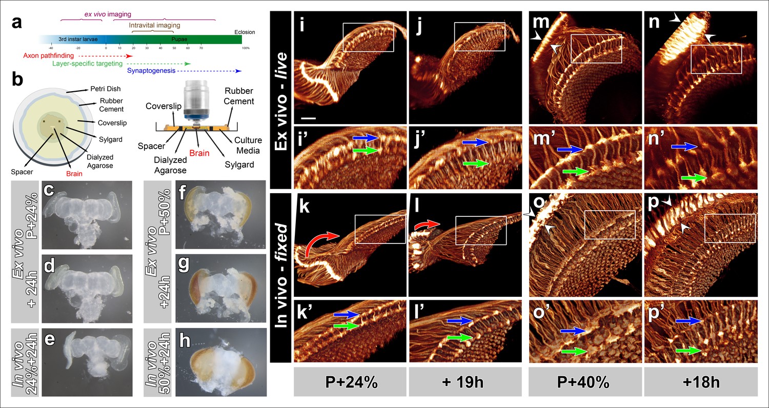
Development of Drosophila pupal brains in an imaging chamber.
(a) Timeline of photoreceptor circuit formation during brain development and the periods accessible by live imaging. (b) Ex vivo imaging chamber, top (left) and side (right) views (see Figure 1—figure supplement 1 for step-by-step assembly). (c-h) Changes in brain morphology during development ex vivo v. in vivo. (c,f) Pupal brains dissected at P + 24% and P + 50%. (d,g) The same brains after 24 hr of development ex vivo. (e,h) Brains that were dissected from pupae collected at P + 24% and P + 50% and aged in parallel to the ex vivo brains. See Figure 1—figure supplement 2 for comparison with free-floating cultures. (i-p) Optic lobe development ex vivo v. in vivo (i’-p’) magnified details of (i-p). All photoreceptors express CD4-tdGFP. Initial layer separation (P + 24% + 19 hr) occurs ex vivo (i’,j’) similarly to the in vivo controls (k’, l’) aged in parallel (blue arrows: R8, green arrows: R7). Lamina rotation (red arrows) observed in vivo (k, l) is defective ex vivo (i, j). Final layer formation and lamina expansion (P + 40% + 18 hr) occurs similarly ex vivo and in vivo, (m’-n’) v. (o’-p’) (arrows) and (m-n) v. (o-p) (between arrowheads), respectively. Note that for the ex vivo brains, images of the same specimens were taken at different time points, while for the in vivo controls different brains had to be fixed and imaged for the different time points. Scale bars, 20 μm.
Figure 1—figure supplement 1
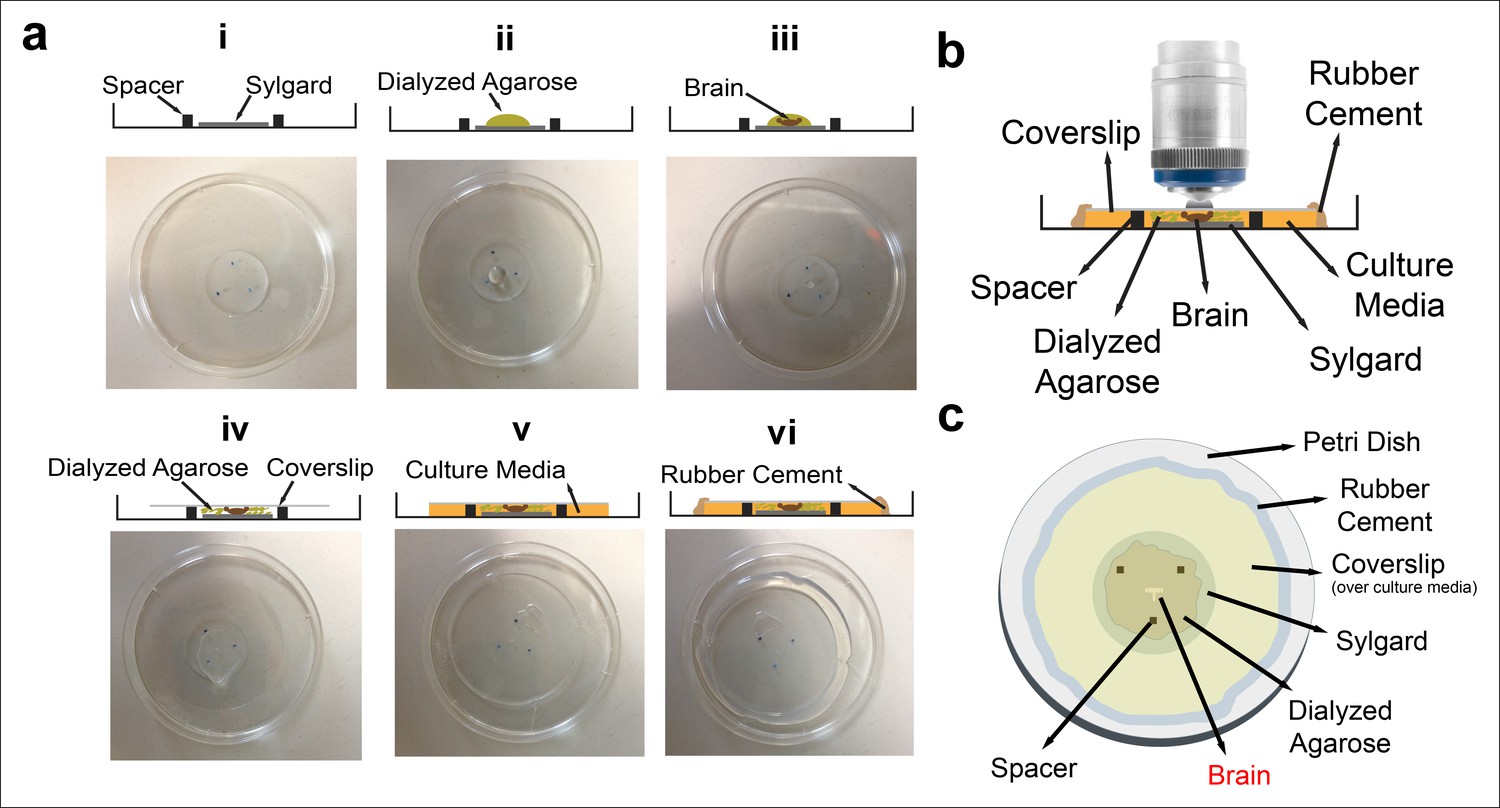
Culture imaging chamber.
(a) Step-by-step construction of the imaging chamber. (i) Spacers are placed on the Sylgard layer in a triangle formation. (ii) A drop of diluted dialyzed agarose is pipetted onto the Sylgard. (iii) Dissected eye-brain complex is placed into the agarose drop. (iv) The mix is covered with a coverslip. (v) After the agarose polymerization, remaining space under coverslip is filled with the culture media; (vi) and sealed completely with rubber cement. The schematic of the final chamber (b) from the side and (c) the top.
Figure 1—figure supplement 2
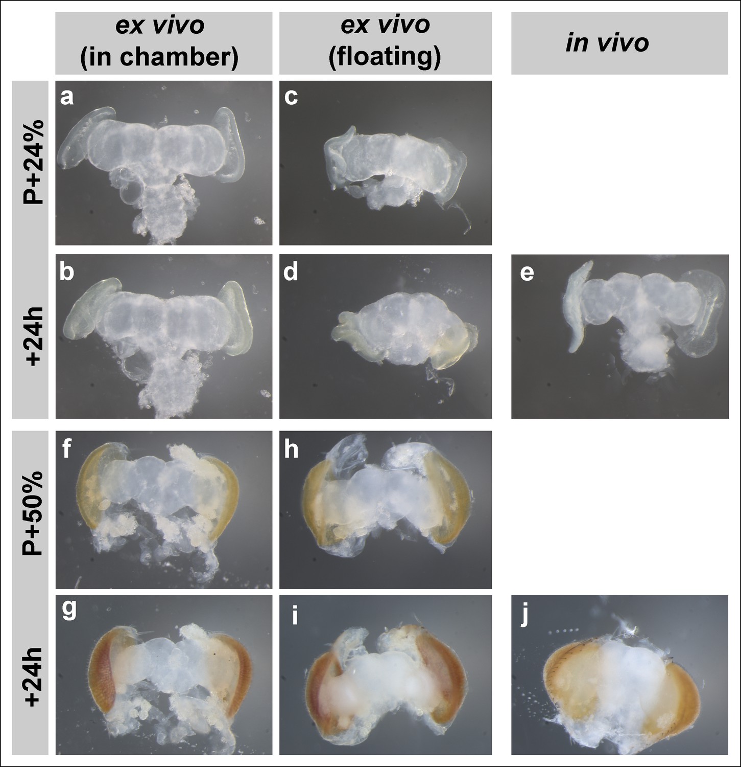
Brain development in imaging chamber compared to liquid media.
Changes in brain morphology during development ex vivo in chamber vs. ex vivo in liquid media (free floating) vs. in vivo; from brains dissected at P + 24% (a-d), P + 50% (f-i) and cultured for 24 hr. Parallel developed in vivo controls (e, j) were dissected at the end of cultures. At early stages, brains that developed in the imaging chamber (b) are more similar in morphology to the in vivo controls (e) than the brains that developed in fully liquid media (d).
Figure 2 with 2 supplements
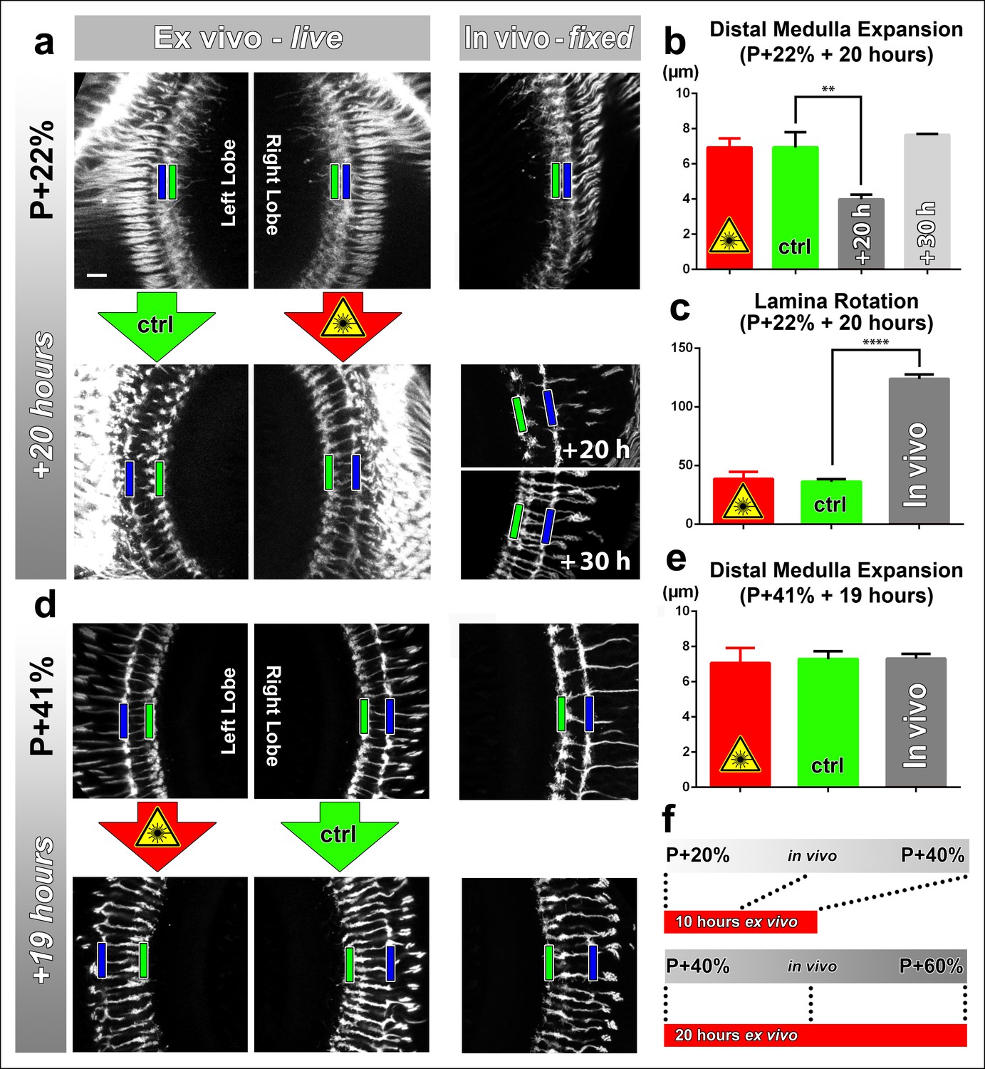
Effects of culture conditions and laser scanning on the optic lobe development ex vivo.
Two-photon imaging of the medulla was performed with brains cultured at P + 22% for 20 hr (a) and P + 41% for 19 hr (d) all photoreceptors express CD4-tdGFP. For each experiment one image stack was acquired containing both optic lobes of a brain. Next, only one of the lobes was scanned every 30 min. Finally, another stack was acquired with both lobes. Different brains aged in parallel in pupae have been dissected as in vivo controls. (b) Quantification of the layer distance increase in P + 22% cultures. The distance between R8 (green rectangles in a,d) and R7 (blue rectangles) layers increase identically in scanned and unscanned ex vivo lobes, but higher than the in vivo control (p = 0.0036, n = 3). (c) Quantification of the change in the angle between the planes of posterior lamina and the anterior medulla. Ex vivo lobes rotate similarly but slower than in vivo controls (p <0.0001, n = 3). (e) Quantification of the layer distance increase in P + 41% cultures. All groups show a similar increase in the distance between R8 temporary layer and R7 terminals. Error bars depict SEM. (f) Calibration of the developmental speed in culture to in vivo development, based on distal medulla expansion. Scale bars, 10 μm.
Figure 2—figure supplement 1
Lamina rotation is incomplete ex vivo.
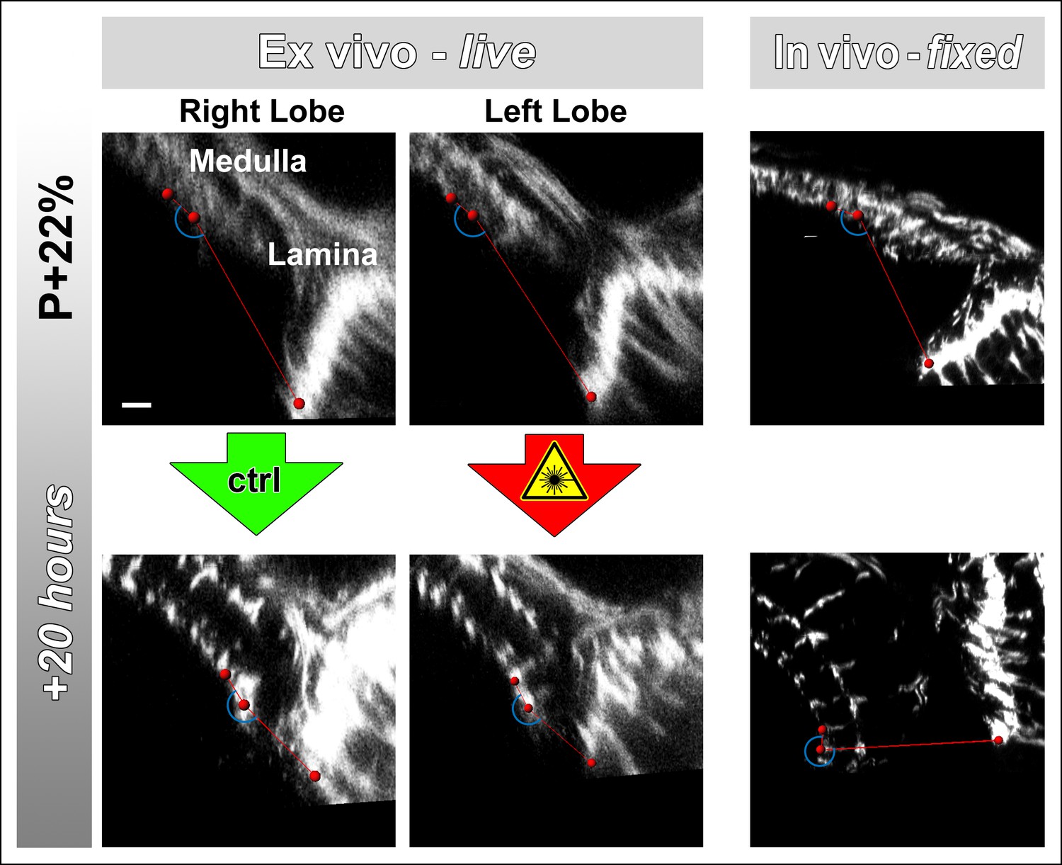
Two-photon imaging of the medulla was performed with brains cultured at P + 22% for 20 hr, all photoreceptors express CD4-tdGFP. Continuously scanned ex vivo culture, unscanned control optic lobe and in vivo (fixed) control experiments were done as described in Figure 2. The angles (blue arches) between the planes of posterior lamina and anterior medulla have been measured for the start and end points of each culture as well as the corresponding in vivo controls; and plotted in Figure 2c. Scale bar, 10 μm.
Figure 2—figure supplement 2
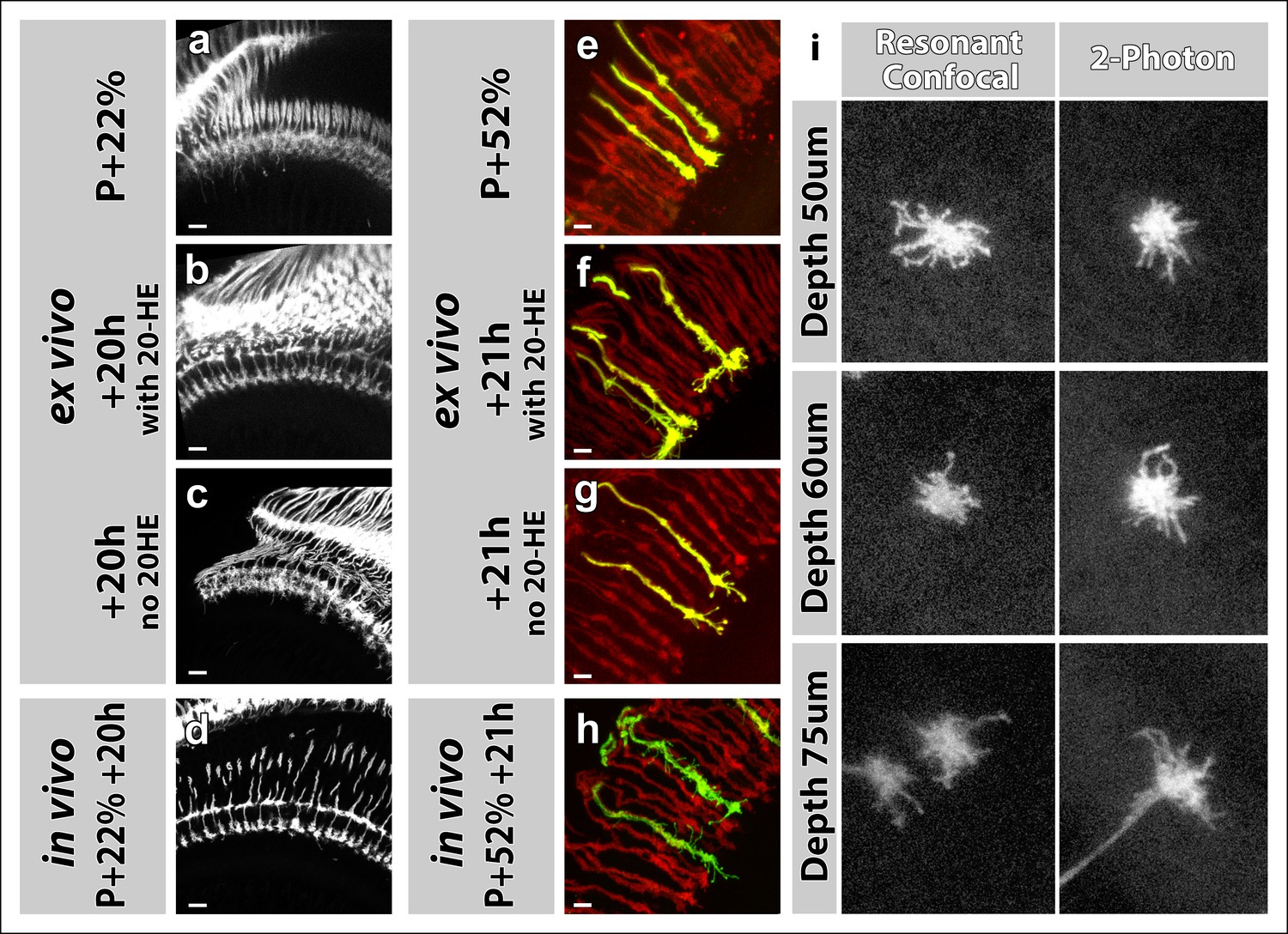
Effects of 20-Hydroxyecdysone (20-HE) and type of microscope on imaging in the culture chamber.
(a-h) 20-HE is required for early but detrimental to late pupal development in the optic lobe. (a-d) All photoreceptors were labeled with CD4-tdGFP. Cultures were set-up at P + 22% (a), with (b) or without (c) 20-HE in the culture media. Parallel developed pupae were dissected and imaged at the end of cultures as in vivo controls (d). R7-R8 layer separation in the medulla was impaired in cultures without 20-HE compared to in vivo controls or cultures with 20-HE. Scale bars, 10 μm. (e-h) All photoreceptors were labeled with td-Tomato and R7 cells were sparsely labeled with CD4-tdGFP using GMR-FLP through MARCM. Cultures were set-up at P + 22% (e), with (f) or without (g) 20-HE in the culture media. Parallel developed pupae were dissected and imaged at the end of cultures as in vivo controls (h). R7 axons that developed in the presence of 20-HE showed excessive filopodial formations on their terminals compared in vivo controls or the cultures without 20-HE. Scale bars, 4 μm. (i) Comparison of resonant confocal and 2-photon microscopy signal stengths in the imaging culture chambes. R7 cells were sparsely labeled with CD4-tdGFP using GMR-FLP through MARCM. Individual R7 growth cones were imaged in the culture chamber at P + 30%. Images were acquired with a Leica TCS SP5 confocal microscope with a resonant scanner or a Zeiss LSM 780 multiphoton microscope at various depths from the coverslip. The confocal signal reduces below 60 μm compared to the 2-photon signal.
Figure 3 with 1 supplement
Different filopodial signatures accompany separate circuit formation steps.
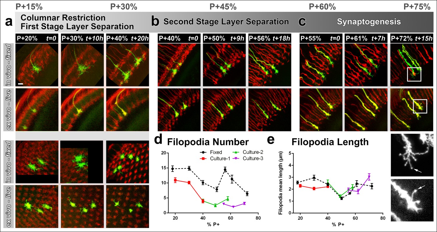
Slow (30 min interval) time-lapse imaging of pupal brains dissected at P + 20% (a), P + 40% (b) and P + 55% (c) in comparison with in vivo fixed controls at the same stages. The same growth cones were analyzed for all live imaging experiments while different samples from parallel aged pupae had to be dissected for the in vivo controls. All photoreceptors were labeled with myr-mRFP and R7 cells were sparsely labeled with CD4-tdGFP using GMR-FLP through MARCM. (a) As the R7 and R8 layers go through their initial separation (upper panel), R7 terminals have numerous filopodia that invade neighboring columns (lower panel), which are pruned around P + 40% both ex vivo and in vivo. (b) As the layers start to reach their final configuration, R7 terminals form a bipartite structure around P + 50%. Filopodia numbers remain low. Around P + 55%, more (shorter) filopodia are observed again as R7 axon assumes a brush-like look. (c) After P + 55% shorter filopodia are pruned and R7 growth cones form new, longer filopodia that are fewer in number and have bulbous tips (arrows). Quantifications of (d) total number of filopodia per growth cone and e, mean length of filopodia through the ex vivo experiments (a-c) and respective in vivo controls. Error bars depict SEM. Scale bars, 5 μm.
Figure 3—figure supplement 1
Filopodial dynamics are restricted to the growth cone and axon shaft inside the medulla neuropil.
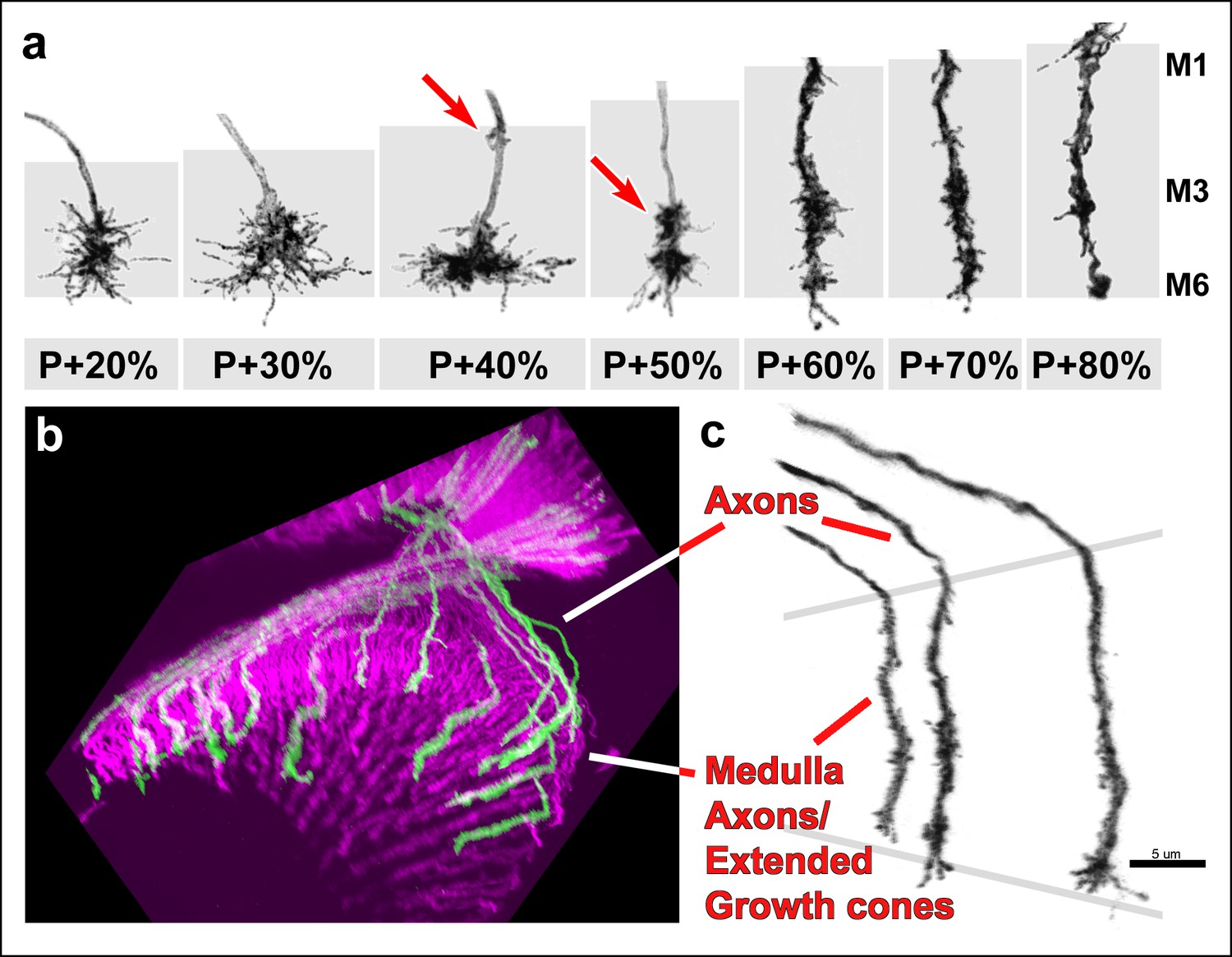
(a) representative R7 terminal structures inside the medulla neuropil (grey background) reveal the transition of a more classical growth cone to a branched axonal structure. (b) 3D visualization of individual R7 axons (green) on the background of all photoreceptors (magenta) at P + 70%. (c) analysis of R7 axons and extended growth cones/axon shafts in the medulla reveals that filopodia only occur within the medulla neuropil.
Figure 4 with 2 supplements
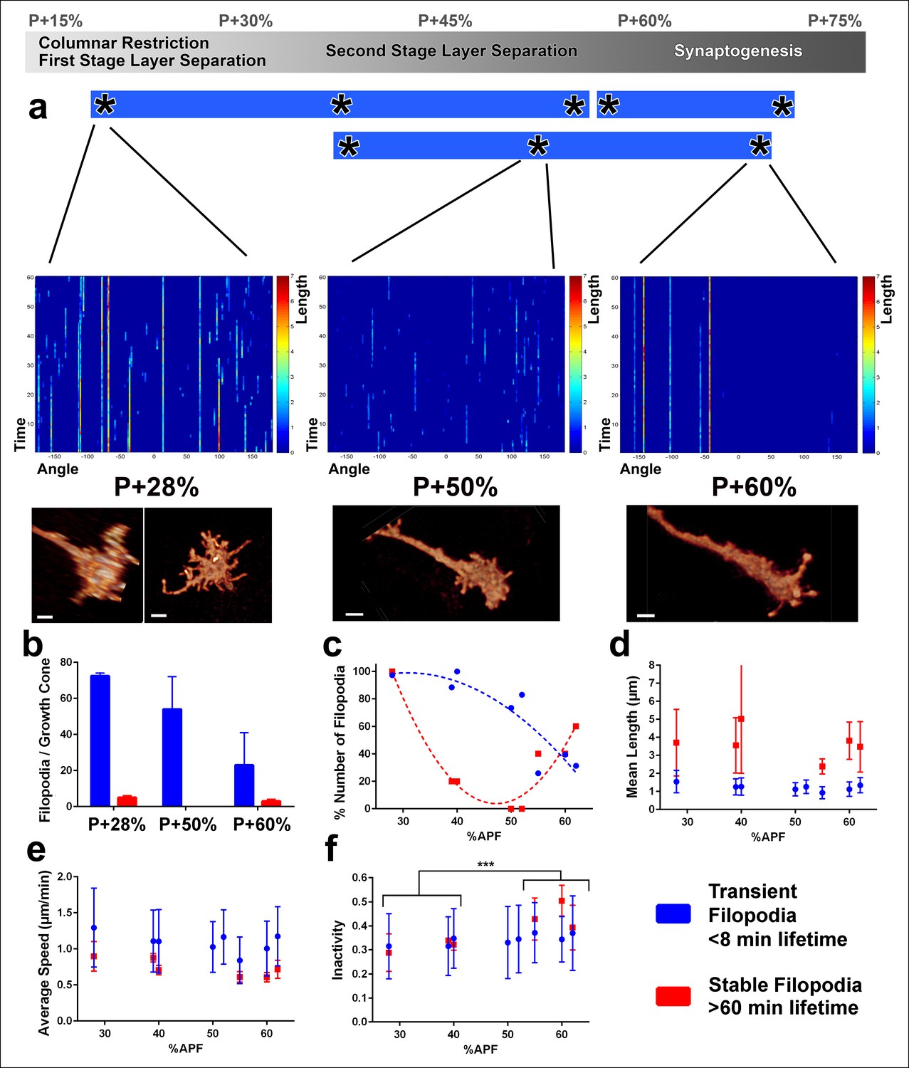
Distinct classes of transient and stable filopodia underlie different developmental events.
Fast (1 min interval) time-lapse imaging was performed at multiple points of three ex vivo experiments. (a) Three time points are shown; during the first-stage (P + 28%) and second-stage (P + 50%) layer formation, and synaptogenesis (P + 60%). 3D graphs (upper panel) show the dynamics of individual filopodia observed in a one hour period. In the heat maps on blue background, individual filopodia are shown as verticals lines. The filopodia were sorted by their initial orientation angle (x-axis). The length of the vertical lines represents the life time of the filopodia (time on the y-axis). The color map indicates the length (μm) for each filopodium through time. Representative images of the growth cones at the above time-points (lower panel). See Figure 4—figure supplement 1 for heat maps and representative images at all time points. (b) Numbers of filopodia per growth cone for the time-points shown in a; for filopodia with lifetime <8 min (transient) and lifetime >1 hr (stable). (c) Numbers of filopodia relative to the numbers at P + 28% for all time-points imaged. Fitted curves: y = 28.17 + 4.597x-0.075x2 (transient) and y = 583.1–24.53x + 0.26x2 (stable). (d) Mean length (μm) (e) Average speed (μm/min) and (f), Inactivity (ratio of intervals with no significant extension or retraction) for transient and stable filopodia at all time-points. Stable filopodia observed after P + 50% have significantly higher inactivity than those observed before (Means: 0.3002 v. 0.4346, p = 0.0002, n = 14 for each). See Figure 4—figure supplement 2 for these parameters as a function of filopodia lifetime on the same growth cone. Error bars depict SD. Scale bars, 2 μm.
Figure 4—figure supplement 1
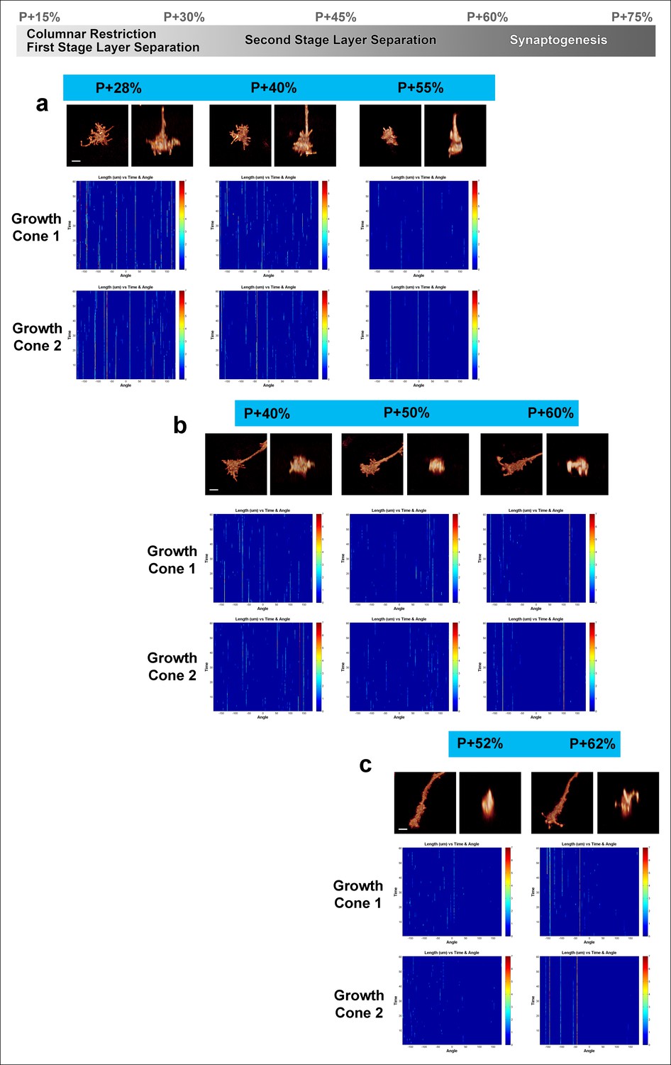
Fast filopodial dynamics throughout pupal development.
Dynamics data from all 6 growth cones (2 independent growth cones for each time point) that were used in Figure 4. The heat maps on blue background show individual filopodia as verticals lines. The filopodia were sorted by their initial orientation angle (x-axis). The length of the vertical lines represents the life time of the filopodia (time on the y-axis). The color map indicates the length (μm) for each filopodium through time. a, starting at P + 28%, after 9 hr in culture and after 19 hr in culture. b, starting at P + 40%, after 8 hr in culture and after 21 hr in culture. (c), starting at P + 52% and 8 hr in culture. Scale bars, 3 μm.
Figure 4—figure supplement 2
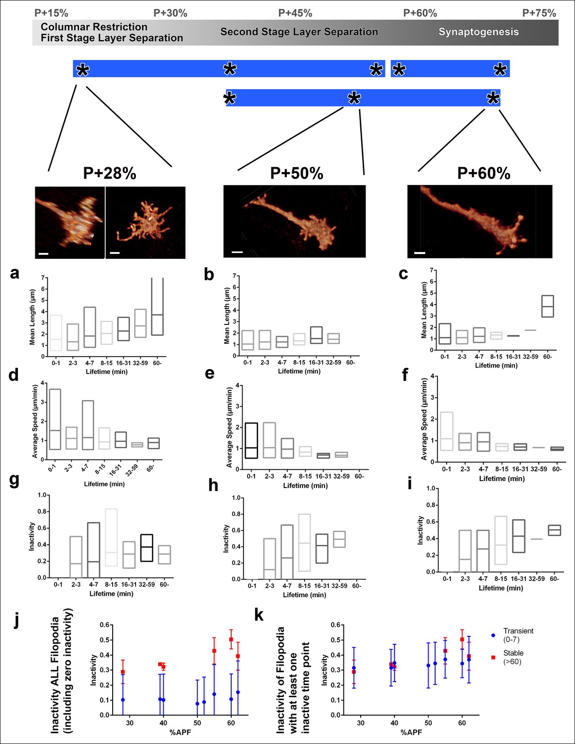
Filopodial dynamics as a function of lifetime.
(a-i) For the same growth cones depicted in Figure 4, every filopodia observed in a 1 hr period were binned into different lifetime classes: <1 min, 2–3 min, 4–7 min, 8–15 min, 16–31 min, 32–59 min or >60 min. Mean length (a-c), speed (d-f) and inactivity (g-i) were plotted for each group of the three growth cones. The boxes cover the entire range and horizontal lines show the mean. Scale bars, 2 μm. (j-k), Mean inactivity (ratio of intervals with no significant extension or retraction) for transient ( <8 min) and stable ( >60 min) filopodia at all time-points. (j), Inactivity: due to the high ratio of filopodia with ‘zero’ inactivity in transient filopodia (g-i), average inactivity appear much lower for transient filopodia. (k) Inactivity of filopodia with at least one inactive time point: after the exclusion of ‘zero inactivity’ filopodia, inactivity of transient and early stage stable filopodia are identical. Error bars depict SD.
Figure 5 with 1 supplement

R7 growth cones do not actively extend in the medulla.
(a) R7 may reach its final target layer through active extension or passive displacement and intercalation. (b) Live imaging starting at P + 30%. All photoreceptors were labeled with myr-mRFP and R7 cells were sparsely labeled with CD4-tdGFP using GMR-FLP through MARCM. R7 growth cone (triangle) initially has a cone structure. As the layer formation progresses, a new varicosity (arrow) is formed from the axon shaft. This structure expands further and by P + 50% the entire terminal thickens. See Figure 5—figure supplement 1 for all time points. (N = 31). (c) Live imaging starting at P + 42%. Both R7 and R8 cells were sparsely labeled with CD4-tdGFP using hsFLP. R7 axon has already formed its distal varicosity (arrowhead); the R8 axon has extended a single filopodia proximally (arrow). Later, this filopodia reaches to the R8 final layer and forms the new terminal. R7 terminal shows no active extension activity. (N = 17 for R7 and 15 for R8). (d) Model of layer formation in the distal medulla. After their arrival to the medulla R7 and R8 terminals are initially separated by intercalation of lamina cell (LM) axons. After P + 40%, R8 growth cones actively extend to new layer while R7s remain in their arrival layer throughout. Scale bars, 3 μm.
Figure 5—figure supplement 1
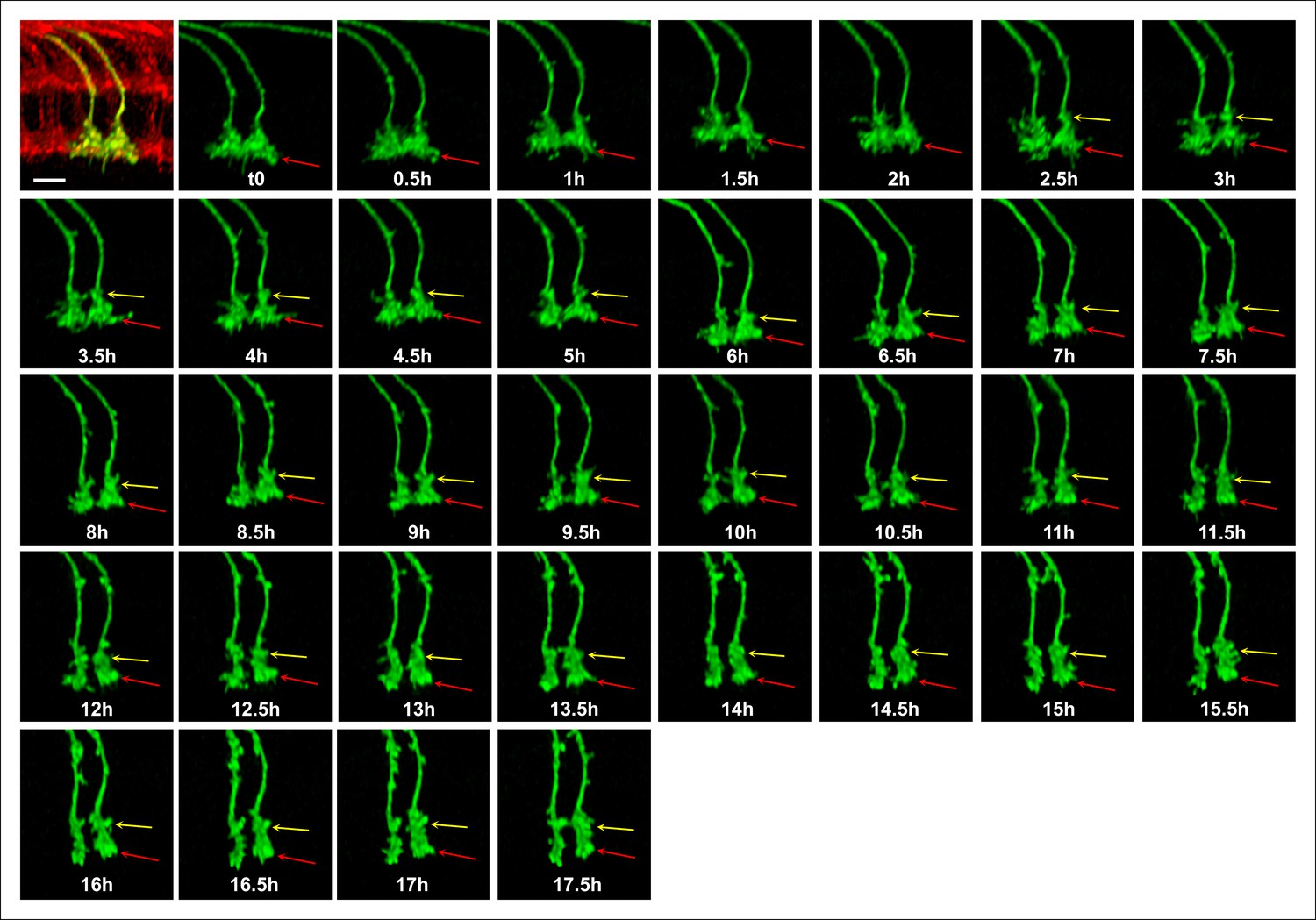
Single growth cone tracking demonstrates R7 terminals remain passive throughout layer formation without a stationary landmark.
Live imaging starting at P + 30%. All photoreceptors were labeled with myr-mRFP and R7 cells were sparsely labeled with CD4-tdGFP using GMR-FLP through MARCM. R7 terminal (red arrow) can be followed throughout 17.5 hr based on its specific filopodial morphology and dynamics. A new varicosity (yellow arrow) was formed from the axon shaft and expands over the course of 15 hr, pushing the terminal distally. No directed activity was observed at the growth cone tip throughout the imaging period. Scale bar, 5 μm.
Figure 6 with 1 supplement
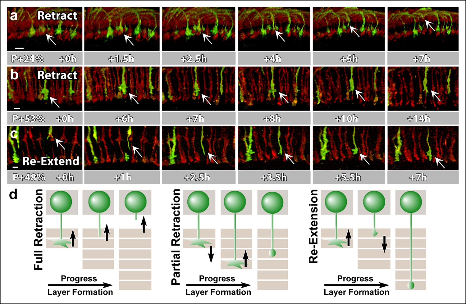
N-Cadherin is required for the stabilization but not the layer specific targeting of R7 growth cones.
All photoreceptors were labeled with myr-mRFP. CadN405 R7 cells were generated with MARCM, using GMR-FLP and positively labeled with CD4-tdGFP. (a) Live imaging started at P + 24% shows a mutant R7 growth cone (arrow) that retracts from its target layer over the course of 5 hr. (b), Live imaging started at P + 53% shows a mutant R7 growth cone (arrow) that retracts from its target layer over the course of 10 hr. Some mutant axons retract completely from the medulla (Figure 6—figure supplement 1) (c) Live imaging started at P + 48% shows an R7 axon (arrow) that has been retracted to the edge of distal medulla but re-extends and attempts to re-innervate both wrong (5.5 hr) and the right (7 hr) layers. (d) Schematics of observed retraction and re-extensions events. Left and middle: Full Retraction leads to complete loss of the R7 axons from the medulla (left), while partial retraction (middle) leads to R7 terminals in an incorrect layer. Number of mislocalized terminals: 33% (n = 85) at P + 40% and 56% (n = 62) at P + 52%. Right: Previously retracted R7 axons can re-extend, even days after they would have been stabilized in wild type. 52% (n = 23) of retracted axons at P + 40% re-extended before P + 50%Scale bars, 5 μm.
Figure 6—figure supplement 1
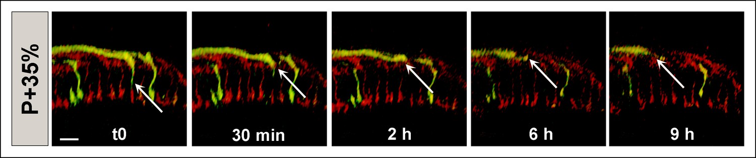
CadN mutant R7 axons may retract completely from the medulla.
All photoreceptors were labeled with myr-mRFP. CadN 405 R7 cells were generated with MARCM, using GMR-FLP and positively labeled with CD4-tdGFP. Live imaging starting at P + 35% demonstrates an R7 axon which retracts from its target layer in the first 2 hr. During the remaining 7 hr, the axon retracts below the R8 temporary layer (upper red layer) and leaves the distal medulla completely. Scale bar, 4 μm.
Figure 7

N-Cadherin is required for fast filopodial dynamics.
CadN405 R7 cells were generated with MARCM, using GMR-FLP and positively labeled with CD4-tdGFP. Fast (1 min interval) time-lapse imaging was performed at P + 28%. (a), The average numbers of filopodia per growth cone are not significantly different between wt and CadN405. (b) Mutant filopodia are slower, (for transient, means wt: 1.303 (n = 143), CadN405: 0.791 (n = 169), p<0.0001; for stable, means wt: 0.898 (n = 10), CadN405: 0.636 (n = 5) p = 0.0199) and (c) shorter (for transient, means wt: 1.542 (n = 143), CadN405: 0.939 (n = 169), p <0.0001; for stable: means wt: 3.707 (n = 10), CadN405: 2.275 (n = 5), p = 0.1257). (d) CadN405 R7 growth cones at the correct layer. Scale bars, 5 μm.
Videos
Video 1
Ex vivo imaging of Drosophila brain development in culture.
All photoreceptors are labeled with CD4-tdGFP. Two live imaging sessions (30 min intervals) starting at P + 24% (19 hr) and at P + 40% (18 hr) are shown. Four developmental processes (i) lamina rotation (ii) lamina column expansion (iii) first-stage separation of R7 and R8 terminals and iv) Final layer formation of R7 and R8 terminals, are shown.
Video 2
Long-term ex vivo imaging of R7 photoreceptor growth cone filopodial dynamics.
All photoreceptors are labeled with myr-tdTomato and R7 photoreceptors are sparsely labeled with CD4-tdGFP using GMR-FLP. Three live imaging sessions (30 min intervals) starting at P + 22% (21 hr), P + 42% (19 hr) and P + 55% (15 hr) are shown. The development of the filopodial structure of R7 growth cones are shown throughout layer and synapse formation.
Video 3
Ex vivo imaging of fast filopodial dynamics-1.
All photoreceptors are labeled with myr-mRFP and R7 photoreceptors are sparsely labeled with CD4-tdGFP using GMR-FLP. Live imaging started P + 28% and continued for 20 hr. We used an alternating slow (30min intervals) imaging of the general structure and fast (1min interval) imaging of two growth cones at higher resolution at three different time points. Fast filopodial dynamics of the same two growth cones at P + 28%, P + 40% and P + 55% are shown.
Video 4
Ex vivo imaging of fast filopodial dynamics-2.
All photoreceptors are labeled with myr-mRFP and R7 photoreceptors are sparsely labeled with CD4-tdGFP using GMR-FLP. Two live imaging sessions starting at P + 40% (22 hr) and P + 52% (9 hr) are shown. We used an alternating slow (30 min intervals) imaging of the general structure and fast (1 min interval) imaging of two growth cones at higher resolution at different time points. Fast filopodial dynamics of the same two growth cones at P + 40%, P + 50% and P + 60% and fast filopodial dynamics of another three growth cones at P + 52% and P + 62% are shown.
Video 5
Second stage layer targeting of R7 and R8.
Two live imaging experiments are shown. (1) All photoreceptors are labeled with myr-mRFP and R7 photoreceptors are sparsely labeled with CD4-tdGFP using GMR-FLP. Imaging started at P + 30% and continued for 18 hr, with 30 min intervals. Two R7 growth cone tips (red arrow) were followed. At the 2.5 hr mark a varicosity starts to develop from the axon shaft and expands over the next 15 hr, contributing to the elongation of the R7 axon. Note that being able to follow the same growth cone tip based on its unique filopodial structure allows us to verify lack of active extension without a stationary landmark. (2) R7 and R8 photoreceptors were sparsely labeled with CD4-tdGP using hs-FLP. Imaging started at P42% and continued for 21 hr. We used an alternating slow (30 min intervals) imaging of the general structure and fast (1 min interval) imaging of two neighboring R7 and R8 growth cones at higher resolution at different time points. R8 axon relocates to its final layer by sending a single filopodia proximally, which is initially very dynamic but later stabilizes and expands in the new layer, forming the new R8 terminal. In contrast, R7 terminal elongates along the axon shaft, but no directed extension activity is observed on the growth cone.
Video 6
N-Cadherin functions in growth cone stabilization.
All photoreceptors are labeled with myr-mRFP and approximately 10% of R7 photoreceptors were made mutant for CadN and labeled with CD4-tdGFP using GMR-FLP through MARCM. Three live imaging sessions are shown. (1) Starting at P + 24% (17 hr). R7 axons arrive correctly to their target layer but they gradually retract from it, preceded by growth cone collapse. (2) Starting at P + 53% (20 hr). Retractions continue despite the wild-type photoreceptors reached their final layer configurations. (3) Starting at P + 42% (11 hr). Some of the R7 axons that retracted at the earlier stages re-extend back into the distal medulla. Note that the growth cones are streamlined during active movement but show expansion while the axons attempt to re-innervate various medulla layers.
Video 7
Loss of N-Cadherin leads to reduced filopodial dynamics.
Representative wild type and cadN mutant R7 growth cones are shown at P + 28%. Extraction of individual filopodia reveals reduced dynamics over the same time period (1 hr with 1 min time lapse) as shown in the quantifications in Figure 7.
Additional files
-
Source code 1
The MATLAB function for analysis of the filopodial dynamics.
This function takes as input the Excel files including the length and orientation data for all filopodia segmented across 60 time points within a 1 hour period. "TrackID"s are also required to identify the same filopodia across different time points. The function then calculates for each TrackID the number of extension and retraction events it experienced during that filopodium's lifetime, as well as the mean and standard deviation for extension, retraction and combined speeds. The user is asked for an input (in μm) defining the amount of extension/retraction length (default=0.3 μm) that will be considered insignificant, i.e. the filopodium will be assumed static for that 1 minute step. The function then outputs the number of extension and retraction events above that threshold ("filtered"), as well as speeds calculated from only these (above-threshold) events. The function also calculates the mean and standard deviation of a filopodium's length (μm) during its lifetime. These parameters are written in a new Excel file. Finally, the function creates the heat-maps used (and explained) in Figure 4.
- https://doi.org/10.7554/eLife.10721.026
Download links
A two-part list of links to download the article, or parts of the article, in various formats.
Downloads (link to download the article as PDF)
Open citations (links to open the citations from this article in various online reference manager services)
Cite this article (links to download the citations from this article in formats compatible with various reference manager tools)
Filopodial dynamics and growth cone stabilization in Drosophila visual circuit development
eLife 4:e10721.
https://doi.org/10.7554/eLife.10721


