Propagated infra-slow intrinsic brain activity reorganizes across wake and slow wave sleep
- Washington University in St. Louis, United States
- Christian-Albrechts-Universität zu Kiel, Germany
- Goethe-Universität Frankfurt am Main, Germany
Figures
Figure 1
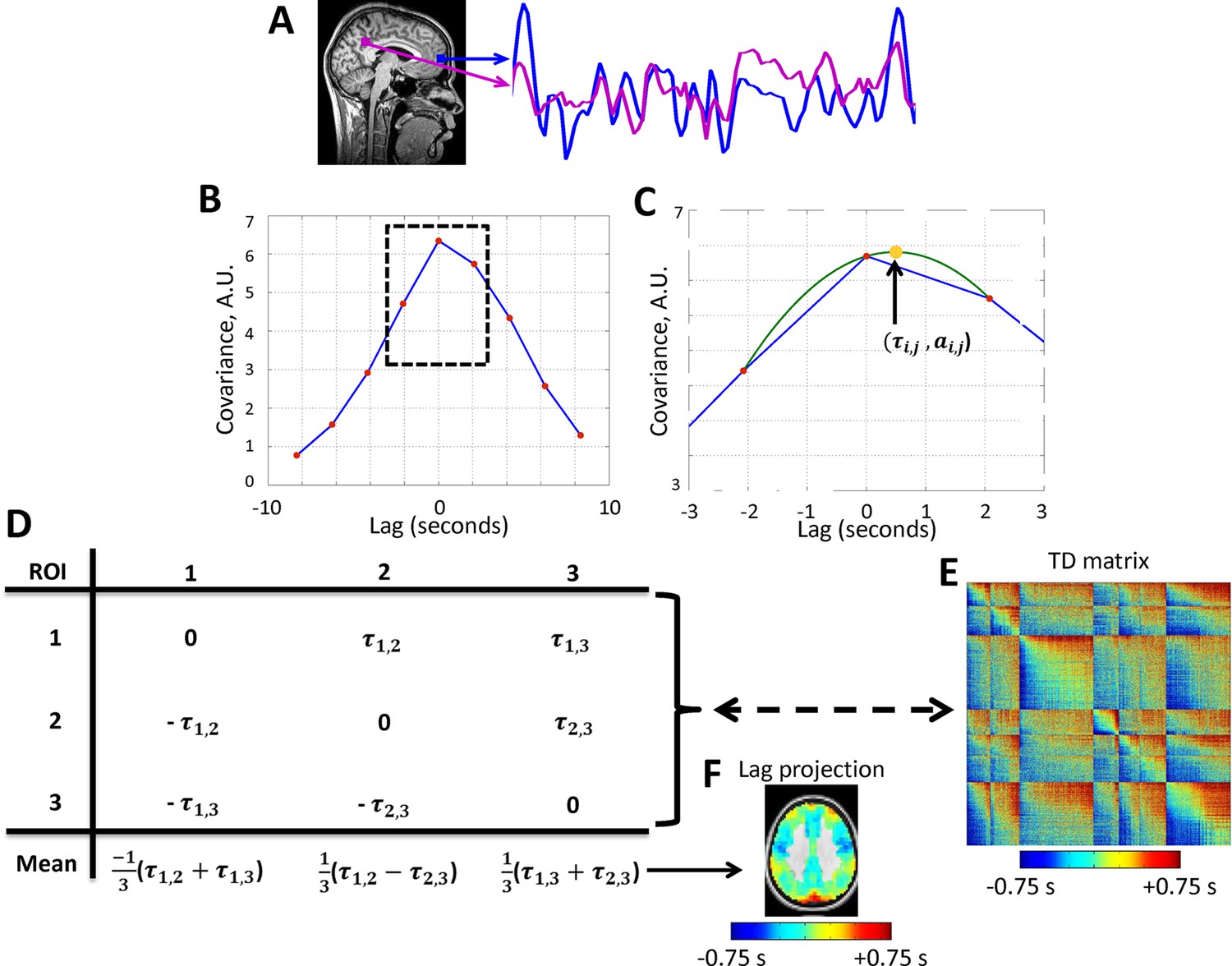
Calculation of lag structure using lagged cross-covariance functions and parabolic interpolation.
Lags are defined by analysis of timeseries derived from two loci. (A) Two exemplar loci (both in the default mode network). The time series were extracted from the illustrated loci over ~200 s. (B) The corresponding lagged cross-covariance function (Materials and methods Equation 2). Although the lagged cross-covariance is defined over the range ± , where is the run duration, the range of the plotted values is restricted to ± 8.32 s, which is equivalent to ± 4 frames (red markers) as the repetition time was 2.08 s. The lag between the time series is the value at which the absolute value of the cross-covariance function is maximal. (C) This extremum can be determined at a resolution finer than the temporal sampling density by parabolic interpolation (green line) through the computed values (red markers). This extremum (arrow, yellow marker) defines both the lag between time series and () and the corresponding amplitude (). (D) Toy case illustration of a time-delay (TD) matrix (Materials and methods Equation 3) representing 3 voxels. TD matrices encode the lag between every pair of analyzed voxels and are anti-symmetric by definition. The mean over each column of a TD matrix generates a lag projection map (Methods Equation 4). A TD matrix obtained with real rs-fMRI data and the corresponding lag projection map are shown in panels (E) and (F), respectively. Panels A-D are adapted from Mitra et al., 2014.
Figure 2
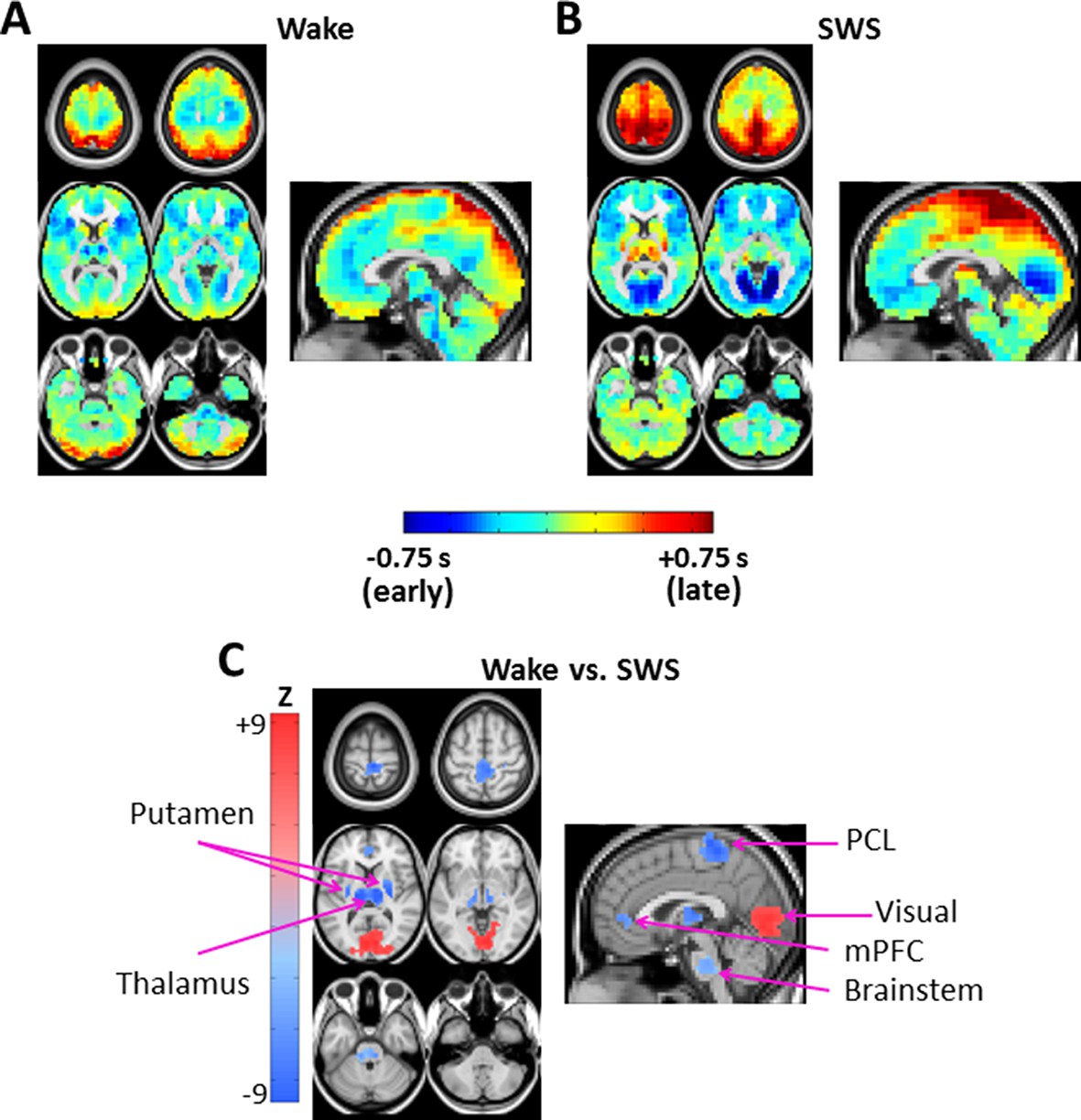
Lag projection maps in wake and slow wave sleep.
Lag projection maps depict the mean lag between each voxel and the rest of the brain (Mitra et al., 2014; Nikolić, 2007). Panels A-B display lag projection maps, in units of seconds, derived from wake (A) and SWS (B). These lag projection maps demonstrate changes in lag structure as a function of state. For example, thalamus is early (blue) during wake but late (red) during SWS; the opposite shift is evident in visual cortex. Panel C shows voxels exhibiting cluster-wise statistical significance in the wake vs. SWS comparison ( > 4.5, p<0.05 corrected). These clusters are centered on putamen bilaterally, thalamus, paracentral lobule (PCL), visual cortex, medial prefrontal cortex (mPFC), and brainstem. Axial slices: Z = +69, +57, +9, -3, -27, -39. Sagittal slice: X = +3.
Figure 3 with 2 supplements
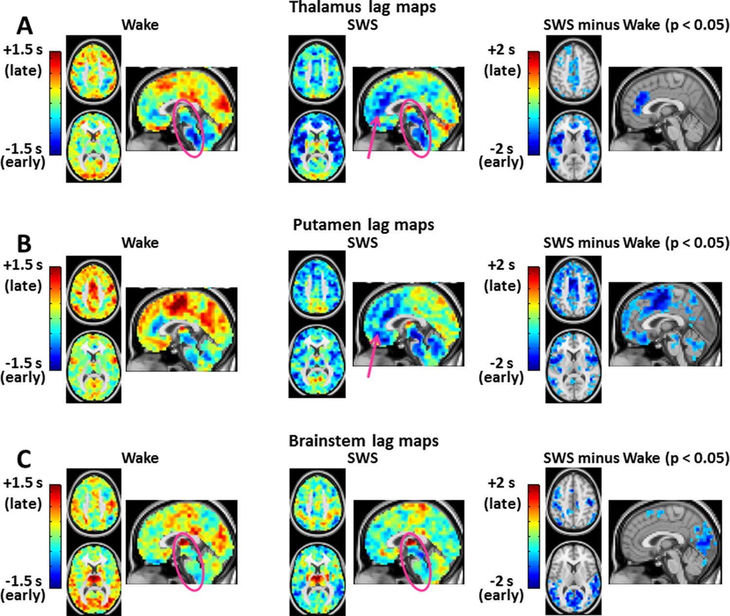
Seed-based lag maps in wake and SWS corresponding to the subcortical regions identified in Figure 2C: thalamus (A), putamen (B), and brainstem (C).
Also shown are lag difference maps (SWS minus wake) thresholded for cluster-wise statistical significance ( Z > 4.5, p<0.05 corrected; as in Figure 2C). During wake, the cerebral cortex is generally late (yellow/red hues) with respect to subcortical regions. The cerebral cortex becomes early (blue/green hues) with respect to subcortical areas during SWS. All significant lag differences are negative (blue), and predominantly found in cortex. Pre-frontal cortex becomes markedly early with respect to the posterior parts of the brain (pink arrows in A and B). This feature suggests a ‘front-to-back’ propagation of slow waves in SWS (Massimini et al., 2004). Lag structure in the brainstem and thalamus is relatively constant (pink ovals in A and C). Lag structure is present within the thalamus in panel A even though the whole thalamus was used as the reference seed. This effect is observed because voxels within large seed-regions, e.g., thalamus, can exhibit non-zero lags with the mean timecourse computed over the entire seed. Axial slices: Z = +45, +9. Sagittal slice: X = +3. An expanded view of these results is shown in Figure 3—figure supplement 1 and 2.
Figure 3—figure supplement 1
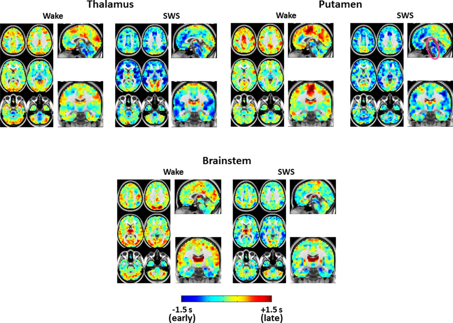
Expanded view of seed-based lag maps derived using thalamus, putamen, and brainstem regions of interest defined in Figure 2C.
Axial and Sagittal slices as in Figure 1. Coronal slice: Y = +12.
Figure 3—figure supplement 2
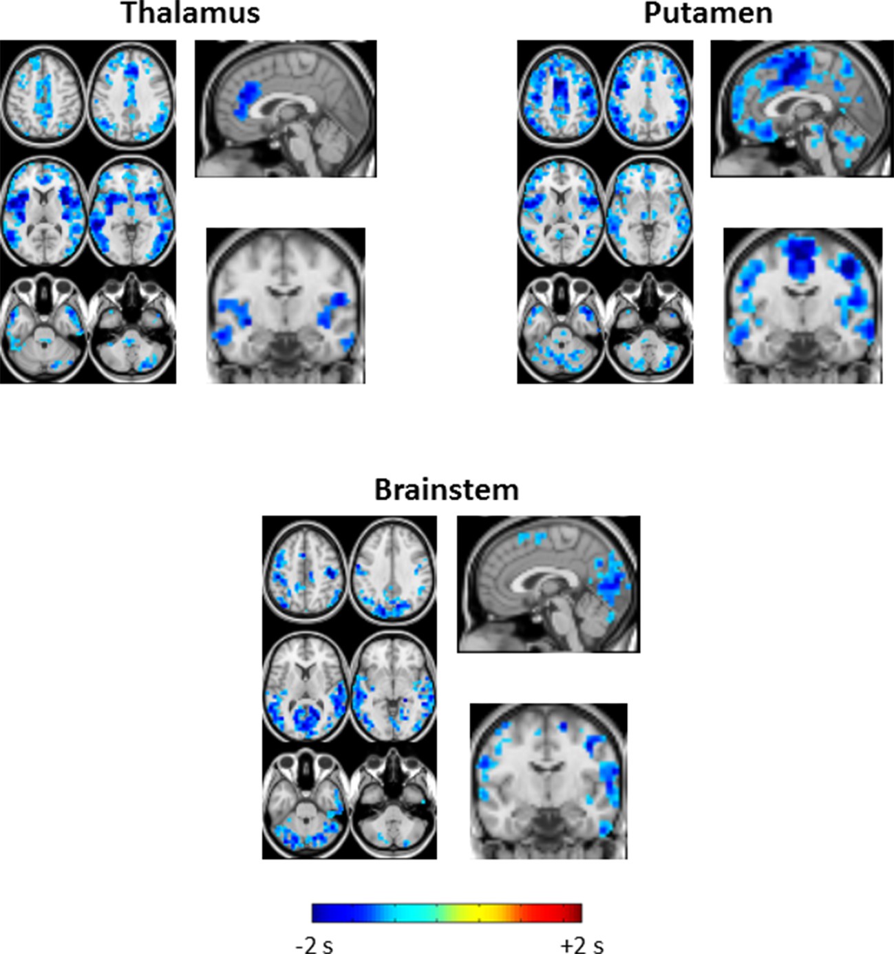
Seed-based lag difference maps thresholded for cluster-wise statistical significance of p<0.05 (as in Figure 2).
All significant lag differences are negative (blue), and predominantly found in cortex, indicating that many areas of cortex become significantly earlier than subcortical structures during SWS as compared to wake. Each of the difference maps also exhibits focality. In particular, thalamus seed lag differences are prominent in anterior cingulate cortex and insula; putamen seed lag differences highlight somatosensory regions and insula; brainstem seed lag differences show that visual cortex becomes markedly earlier than brainstem during SWS.
Figure 4 with 2 supplements
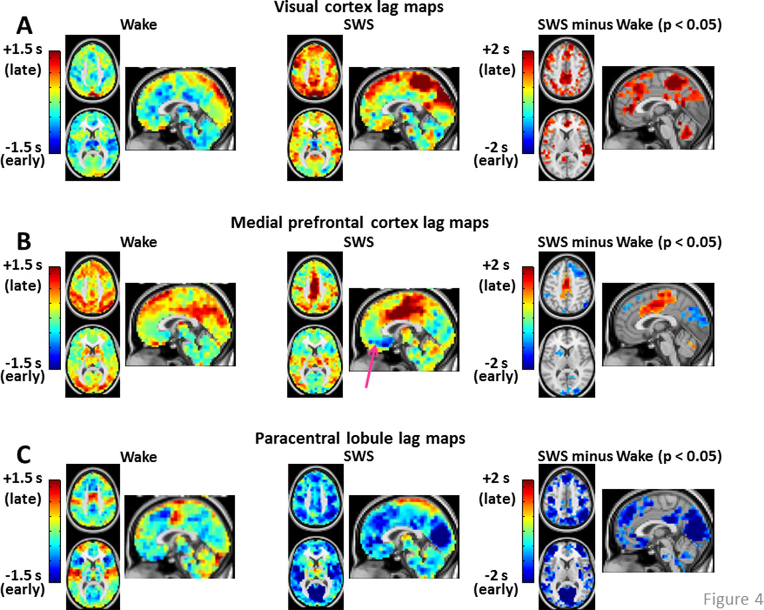
Seed-based lag maps in wake and SWS corresponding to the cortical regions identified in Figure 2C: visual cortex (A), medial prefrontal cortex (B), and paracentral lobule (C).
Also shown are lag difference maps (SWS minus wake), thresholded for statistical significance, as in Figure 2. Panel A shows that, whereas the visual seed is neither wholly late nor early in wake, nearly the entire cortex is late with respect to visual cortex during SWS. Panel B shows that medial prefrontal cortex (mPFC) exhibits both early and late lag shifts between wake and SWS. The mPFC lag map in SWS also exhibits the ‘front-to-back’ propagation pattern highlighted in Figure 3 (pink arrow). Panel C shows that many of the lag relations of the paracentral lobule seed are reversed during SWS relative to wake. For example, in wake, the seed-region leads lateral sensory-motor cortex and posterior insula. These relations reverse in SWS and nearly the entire cerebral cortex becomes early with respect to the paracentral lobule. An expanded view of these results is shown in Figure 4—figure supplement 1 and 2. Slice coordinates identical to Figure 3.
Figure 4—figure supplement 1
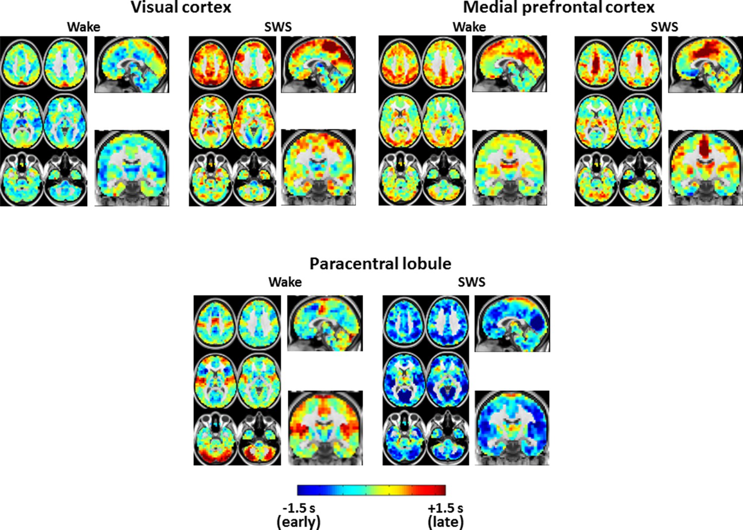
Expanded view of seed-based lag maps derived using visual, medial prefrontal cortex, and paracentral lobule regions of interest defined in Figure 2C.
Slice coordinates identical to Figure 3—figure supplement 1.
Figure 4—figure supplement 2
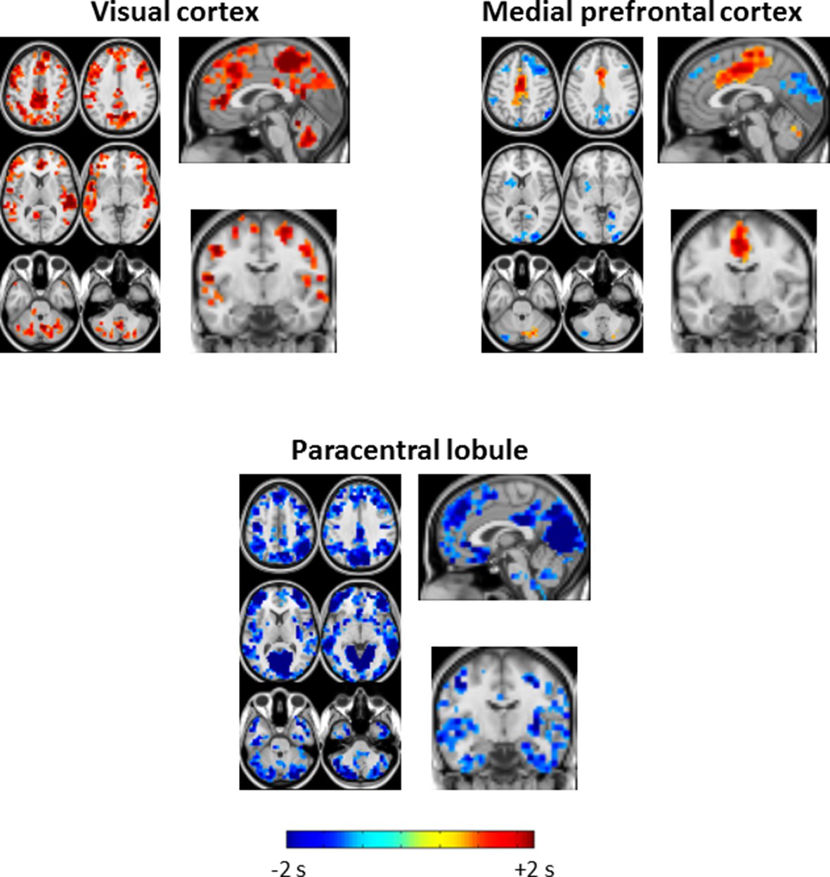
Seed-based lag difference maps thresholded for cluster-wise statistical significance (as in Figure 2).
For the visual cortex seed, nearly the entire cortex becomes late (red) with respect to visual cortex in SWS compared to wake. These effects are especially prominent in paracentral lobule and dorsolateral prefrontal cortex. For the medial prefrontal cortex (mPFC) seed, mPFC exhibits both early and late lag shifts as a function of sleep stage. Occipital and prefrontal areas become earlier (blue) than mPFC during SWS while medial motor structures become later (red). Finally, for the paracentral lobule seed, nearly the entire cortex becomes early (blue) with respect to the paracentral lobule during SWS.
Figure 5 with 2 supplements

Time delay (TD) matrices.
Panels A-B display TD matrices (in units of seconds) in wake and SWS, respectively. Each pixel represents the lag between two voxels. TD matrices are, by definition, anti-symmetric. Hence, all relevant information is contained in the displayed upper triangular values. The matrices displayed in (A-B) have been masked to include only cortical (6 mm)3 voxels with a ≥90% chance of belonging to one of 7 resting state networks (RSNs: dorsal attention network (DAN), ventral attention network (VAN), sensory motor network (SMN), visual network (VIS), frontoparietal control network (FPC), language network (LAN), default mode network (DMN)) ((Hacker et al., 2013), see Figure 5—figure supplement 2). The same RSN definitions are applied in wake and SWS. After sorting voxels by RSN membership, voxels were sorted from early to late within RSN in the wake state. The wake ordering was applied to the SWS TD matrix. Panel C shows the Spearman rank order correlation between wake and SWS lag values in each of the 28 intra- and inter- RSN blocks in panels (A-B). The diagonal blocks in panel C exhibit high correlation values, indicating that intra-RSN propagation is relatively preserved across wake and SWS. The correlation values in the off-diagonal blocks in panel C are low, demonstrating that inter-RSN propagation is strongly altered during SWS. White asterisks indicate significant (p<0.05) effects computed by permutation resampling, including correction for multiple (N = 28) comparisons. Panel D plots the mean within-block values of the wake TD matrix shown in panel A. The values in panel D (in units of sec) are very near zero, implying that no RSN is entirely leads or follows other RSNs. Panel E plots the mean within-block values of the SWS TD matrix shown in panel B. Note significant visual network earliness with respect to other networks (p<0.05 by permutation resampling, multiple comparisons corrected for 21 upper diagonal blocks). Owing to anti-symmetry, the horizontal blue and vertical orange blocks both represent visual earliness. Diagonal blocks in panels D and E are colored gray to symbolize that they are constrained to be zero-mean. TD matrices with alternate voxel orderings are shown in Figure 5—figure supplement 1.
Figure 5—figure supplement 1
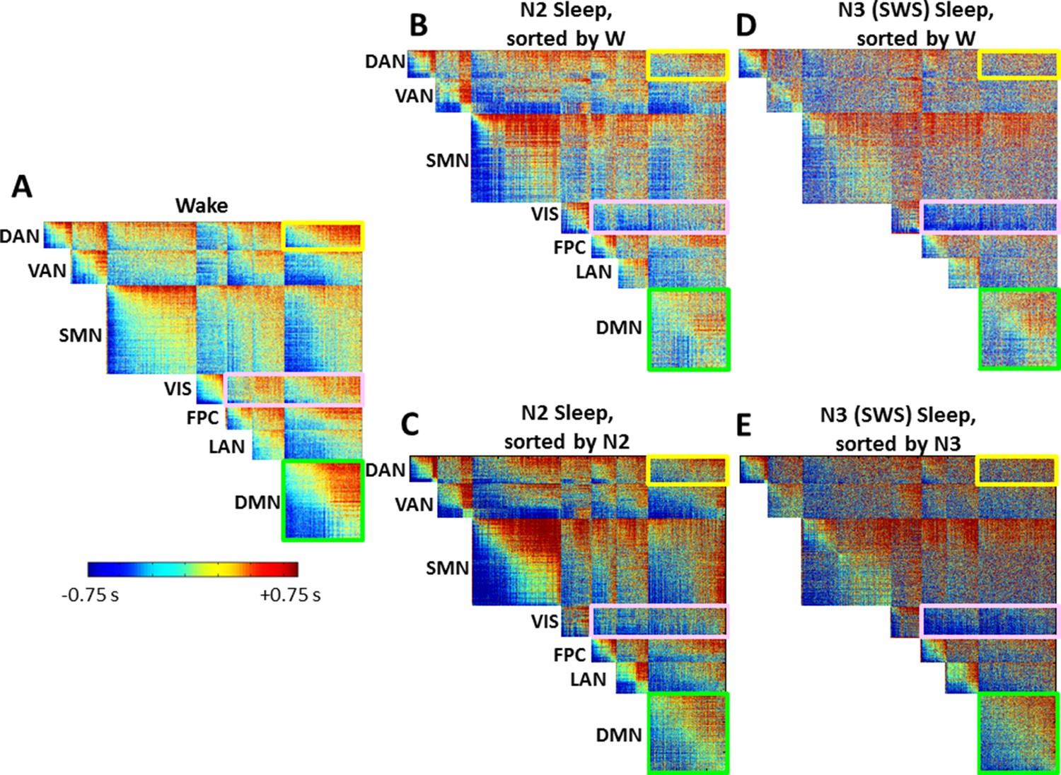
Time delay (TD) matrices as a function of sleep stage, alternate voxel orderings.
(A) Wake. (B-C) N2 sleep. (D-E) N3 sleep (SWS). Panels A and D duplicate panels A and B in Figure 5. Panels C and E provide an alternative view of cross-RSN lag structure disorganization during sleep. In both Figure 5 and here, voxels are ordered first by RSN membership and, within RSN, by lag computed using the projection method. In Figure 5, voxel ordering was determined according to the wake lag structure. Here, in panels C and E, voxel ordering was determined by the stage-specific lag structure, i.e., N2 and N3, respectively. Panels C and E demonstrate that the results shown in main text Figure 5 are robust to the alternative voxel ordering. Specifically, (1) intra-RSN lag structure (diagonal blocks) is generally preserved in all TD matrices, as illustrated by the DMN block highlighted in green; (2) Most inter-RSN (off-diagonal) blocks exhibit increasingly disorganized lag structure in N2 and N3 sleep, as in the DAN:DMN block, highlighted in yellow; (3) The visual network, highlighted in pink, assumes an ‘all early’ organization with respect to other cortical RSNs.
Figure 5—figure supplement 2
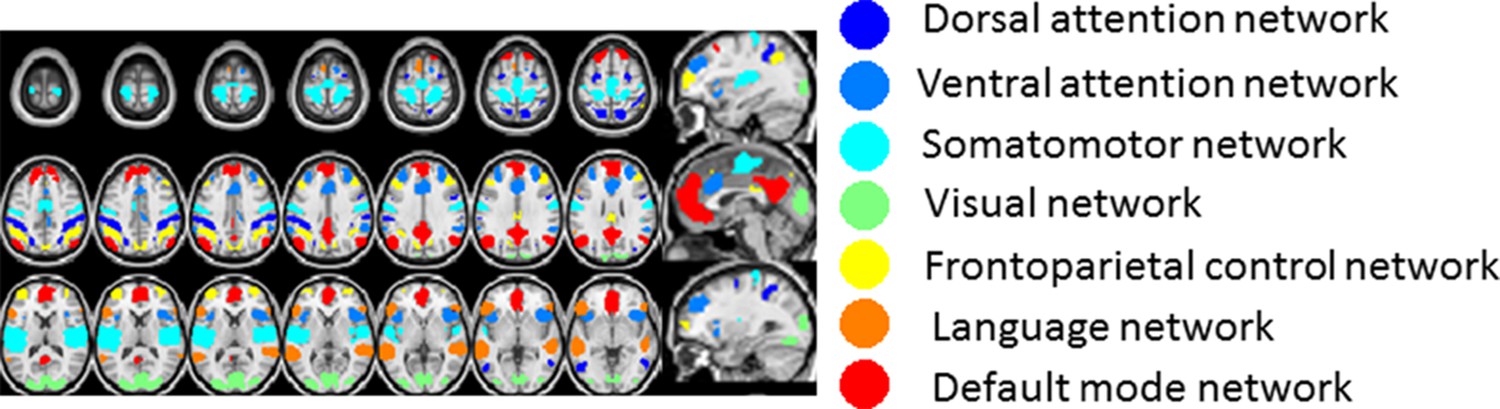
Resting state network (RSN) assignments for gray matter voxels used to compute the TD matrix and functional connectivity matrix results shown in main Figures 5, 6.
This figure illustrates the 1065 (6 mm)3 gray matter voxels satisfying a criterion of ≥90% probability of belonging to one of the 7 cortical resting state networks defined in (Hacker et al., 2013). The color code in this figure is unrelated to latency. The lag maps shown in main text Figures 2–4 are based on a parcellation of the entire gray matter into 6526 (6 mm)3 voxels.
Figure 6
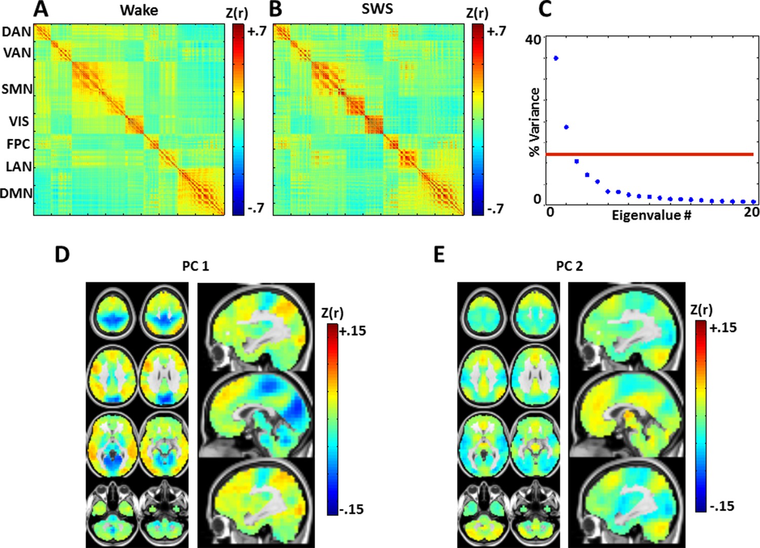
Zero-lag correlation (conventional functional connectivity; FC) matrices.
(A): wake. (B): slow wave sleep. Voxels shown in the correlation matrices correspond to Figure 5A, B (see also Figure 5—figure supplement 2), and matrix values are Fisher-z transformed Pearson correlations averaged over subjects. Note relatively preserved RSN organization across states, in line with previous analyses of these data (Tagliazucchi et al., 2013a). To assess the topography of pair-wise correlation changes, we computed the difference between the SWS and wake correlation matrices (wake minus SWS), and applied spatial principal components analysis (PCA) to the difference matrix. The resulting eigenspectrum (panel C) shows that there are 2 statistically significant (p<0.05; red line) PCs (threshold computed by permutation re-sampling). The topographies of these PC's are shown in panels D and E. These topographies reflect modest FC reductions in visual/somatosensory networks in wake vs. SWS, and modest FC increases in the DMN and thalamus in wake vs. SWS. These results are in accordance with previous findings comparing wake vs. NREM sleep (Horovitz et al., 2008; Picchioni et al., 2013). Importantly, zero-lag correlation structure (panels A-B) is much more preserved across wake and SWS than is lag structure (Figure 5). Axial slices: Z = +69, +57, +45, +33, +9, -3, -27, -39. Sagittal slices: X = +3, +12, -12.
Figure 7 with 2 supplements
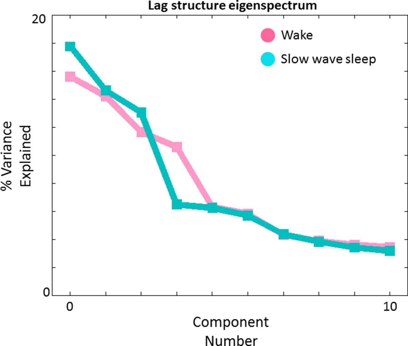
Lag structure dimensionality in wake and SWS.
We have previously shown that multiple temporal sequences can be extracted from a TD matrix by applying spatial principal components analysis (PCA) to the TD matrix after zero-centering each column (Mitra et al., 2015). Here we show PCA-derived eigenvalues (scree plot) obtained in wake (pink) and SWS (blue). The maximum likelihood dimensionality estimates derived using the method of (Minka, 2001) are 4 and 3, respectively, in wake and SWS. The corresponding topographies (‘lag threads’) are shown in Figure 7—figure supplement 1 and 2. N.B.: We previously obtained a maximum likelihood TD dimensionality estimate of 8 in a much larger (N = 688) awake dataset (Mitra et al., 2015). The lower presently obtained figure (4) reflects less statistical power owing to a smaller subject sample (N = 39).
Figure 7—figure supplement 1
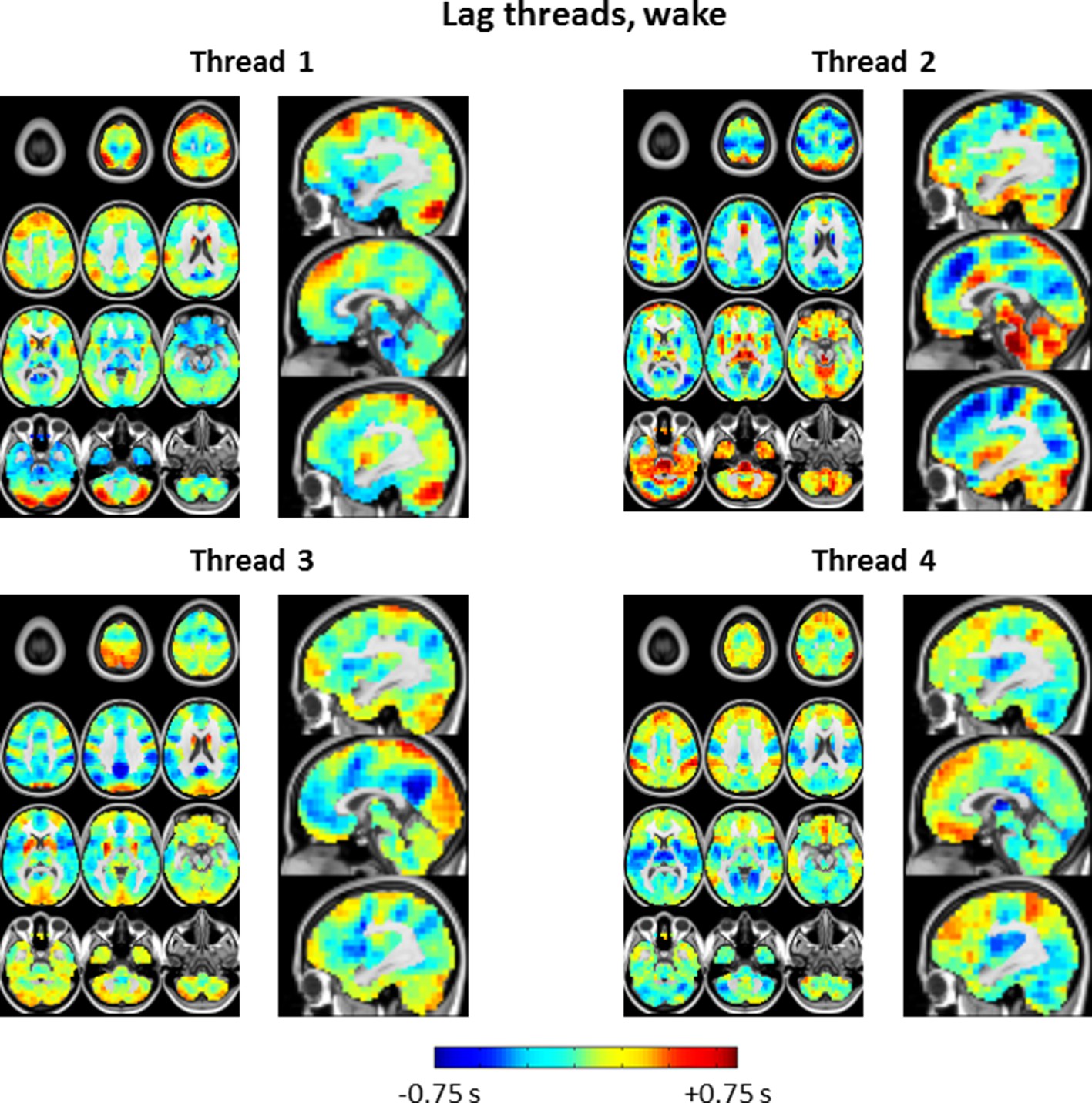
Lag thread topographies in wake corresponding to the eigenvalues shown in Figure 7.
Four lag threads are shown in accordance with the maximum likelihood dimensionality estimate. The illustrated topographies are comparable to the first 4 lag threads shown in Figure 2 of Mitra et al., 2015.
Figure 7—figure supplement 2
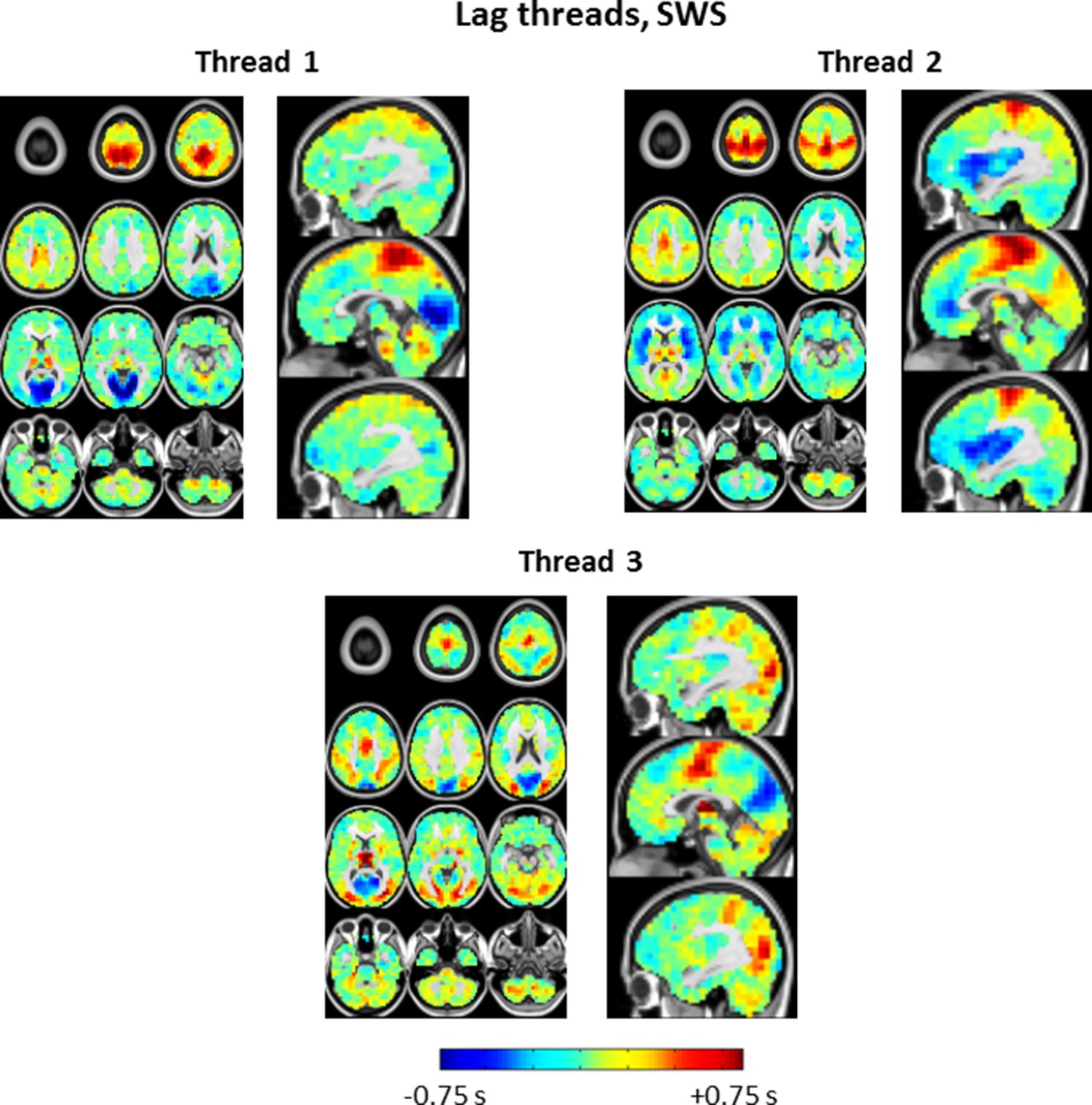
Lag threads topographies in SWS.
Note pronounced differences in comparison to lag threads obtained in wake (Figure 7—figure supplement 1). SWS lag threads 1 and 3 show visual earliness and paracentral lobule lateness, as in Figure 2 and 4. Lag thread 2 shows a front-to-back propagation pattern, in line with main Figures 3, 4 as well as prior electrophysiological results (Massimini et al., 2004).
Download links
A two-part list of links to download the article, or parts of the article, in various formats.
Downloads (link to download the article as PDF)
Open citations (links to open the citations from this article in various online reference manager services)
Cite this article (links to download the citations from this article in formats compatible with various reference manager tools)
Propagated infra-slow intrinsic brain activity reorganizes across wake and slow wave sleep
eLife 4:e10781.
https://doi.org/10.7554/eLife.10781


