The genetic basis for ecological adaptation of the Atlantic herring revealed by genome sequencing
- Uppsala University, Sweden
- University of Macau, China
- BGI-Shenzhen, China
- Qingdao University, China
- Stockholm University, Sweden
- Southeast University, China
- Swedish University of Agricultural Sciences, Sweden
- University of Bergen, Norway
- Hjort Center of Marine Ecosystem Dynamics, Norway
- Institute of Marine Research, Norway
- Texas A&M University, United States
Figures
Figure 1 with 1 supplement
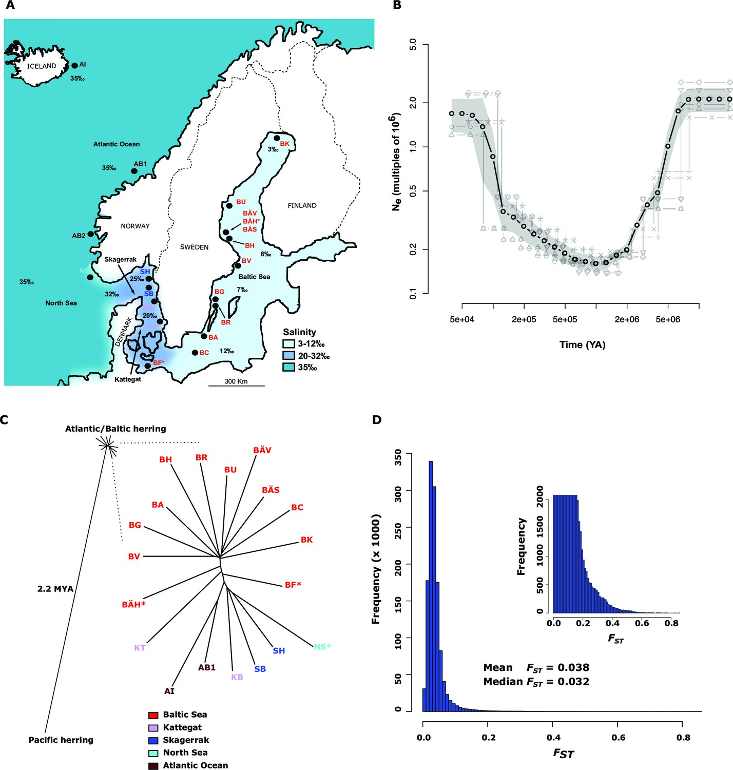
Demographic history and phylogeny.
(A) Geographic location of samples. The salinity of the surface water in different areas is indicated schematically. Autumn spawners are marked with an asterisk. (B) Demographic history. Black circles indicate effective population size over time estimated by diCal (Sheehan et al., 2013); estimates are averages from four arbitrarily chosen genomic regions. The grey field is confidence interval ( ± 2 sd), while light grey lines show the underlying estimates from each genomic region. (C) Neighbor-joining phylogenetic tree. The evolutionary distance between Atlantic and Pacific herring was calculated using mtDNA cytochrome B sequences; right panel, zoom-in on the cluster of Atlantic and Baltic herring populations. Colour codes for sampling locations are the same as in Figure 1A. (D) Global distribution of FST –values based on 19 populations of Atlantic and Baltic herring. The inset illustrates the tail of the distribution. The mean and median of this distribution are indicated. To reduce the FST sampling variance, we only used SNPs with ≥30x coverage in each population.
Figure 1—figure supplement 1
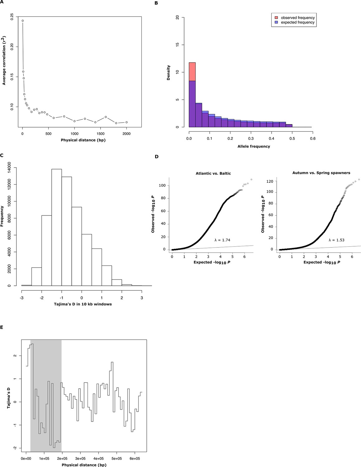
Population genetics and Q-Q plot.
(A) Average decay of linkage disequilibrium estimated from 30 genomic regions of 50 kb each, covering a total of 40,000 SNPs. (B) Comparison between observed and expected distribution of minor allele frequencies in Atlantic herring. (C) Genome-wide distribution of Tajima’s D values, calculated in 10 kb windows (mean =-0.57 ± 0.01). (D) Q-Q plots for the contrasts Atlantic vs. Baltic and spring- vs. autumn-spawners. The inflation factor is slightly higher than 1 for both these distributions which is expected considering that the average genetic differentiation among populations is not zero (mean FST = 0.038, Figure 1D). (E) Tajima’s D values, calculated in 10 kb windows for scaffold 1420 for 16 individually sequenced Atlantic and Baltic herring. The shaded region highlights the putative selective sweep region present in spring-spawning herring (see Figure 4E).
Figure 2 with 5 supplements
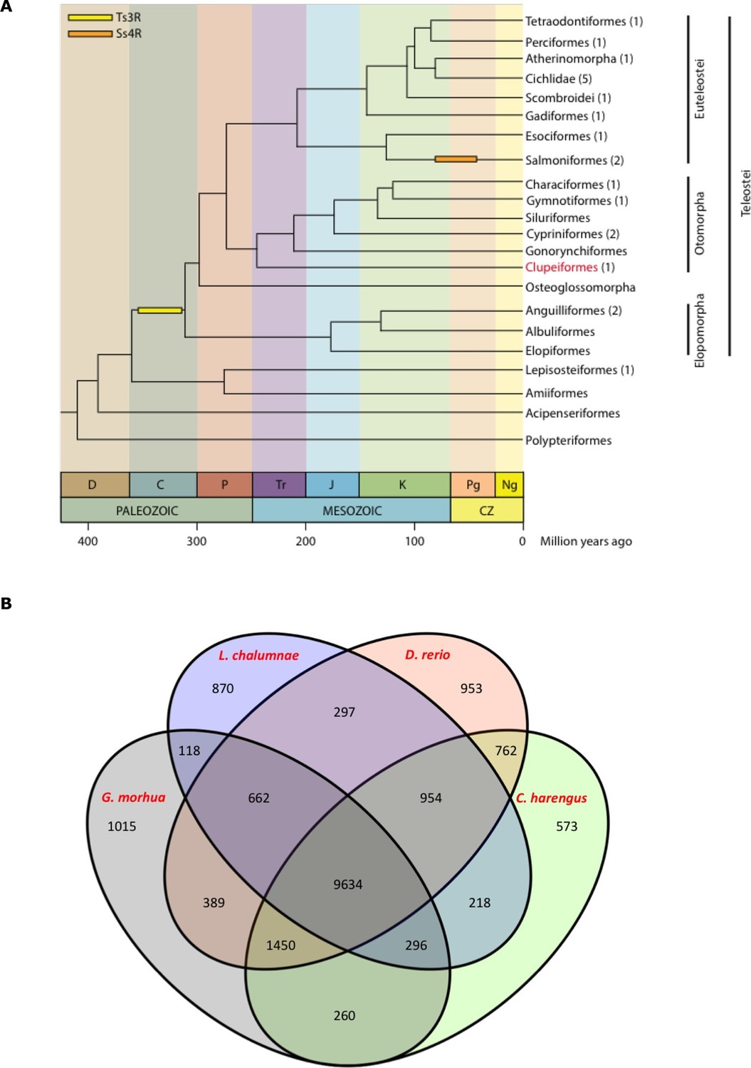
Genome assembly and annotation.
(A) Phylogeny of ray-finned fishes (Actinopterygii) from the Devonian to the present, time-calibrated to the geological time scale based on Near et al. (2012). Geological abbreviations: C (Carboniferous), CZ (Cenozoic), D (Devonian), J (Jurassic), K (Cretaceous), Ng (Neogene), P (Permian), Pg (paleogene) and Tr (Triassic). Dating of the specific rounds of whole genome duplication is based on Glasauer and Neuhauss (2014). Abbreviations: Ts3R (teleost-specific third round) and Ss4R (salmonid-specific fourth round) of duplication. The number of species with a genome assembly available is marked within parentheses after their group’s name. Atlantic herring belongs to Clupeiformes, the order indicated in red letters. (B) Orthologous gene families across four fish genomes (C. harengus, D. rerio, L. chalumnae and G. morhua).
Figure 2—figure supplement 1
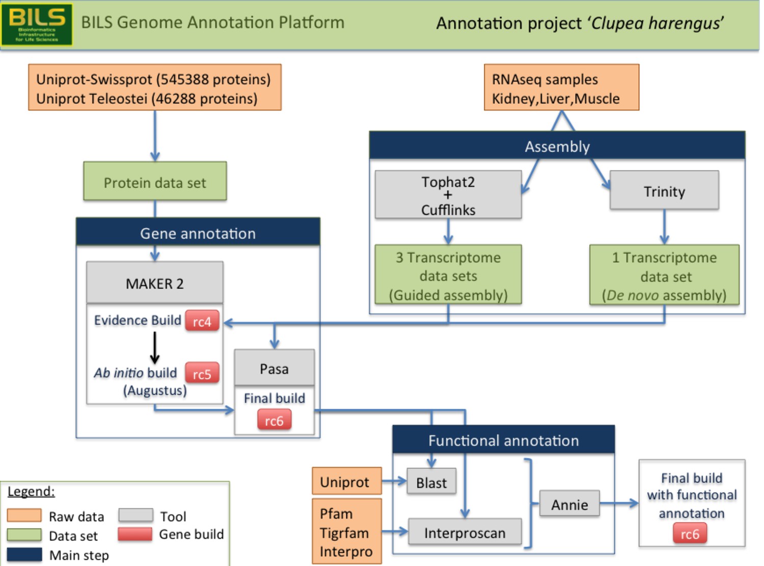
Schematic overview of the annotation pipeline.
Program versions used are detailed in Materials and methods.
Figure 2—figure supplement 2
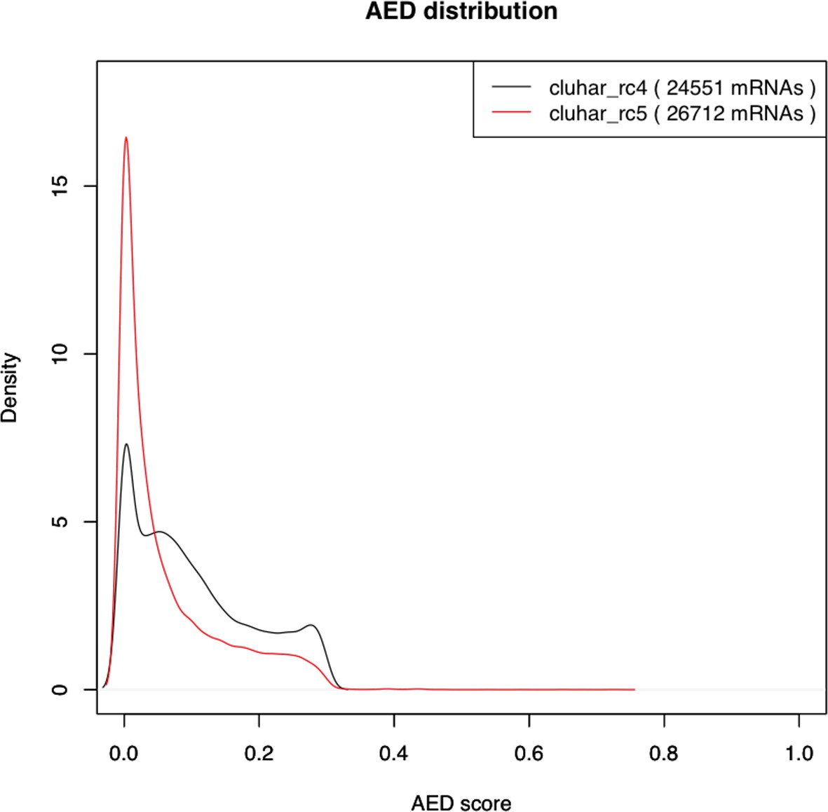
Density plot of the Annotation Edit Distance (AED) score distribution for gene builds rc4 and rc5.
The refined rc5 (red stroke) shows a distribution closer to 0 compared to the evidence build (black stroke), thereby supporting a second pass of ab initio gene modeling that includes in rc5 those genes lacking support from evidence models alone.
Figure 2—figure supplement 3
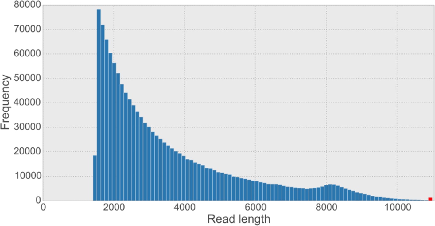
Overall read length histogram for the five synthetic long reads (SLR) libraries.
The shape of the histogram looks similar to other published length histograms (Voskoboynik et al., 2013). The sequence provider has filtered out SLRs shorter than 1,500 bp from the dataset. The red bar indicates the frequency of reads longer than the 99.9% percentile of the data (i.e. 10,887 bp).
Figure 2—figure supplement 4
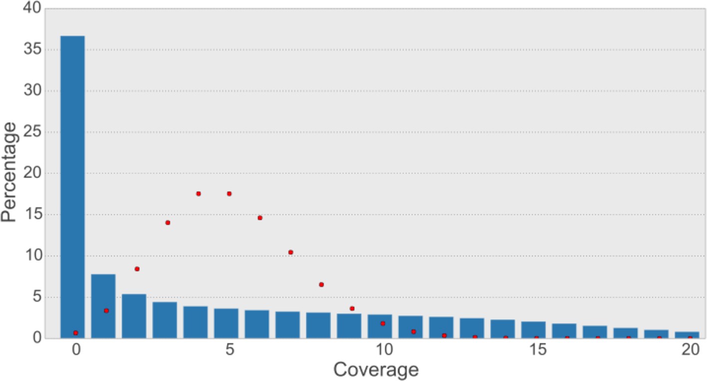
Read coverage of the assembly with synthetic long reads (SLRs) is uneven and not Poisson-shaped.
The average coverage for SLRs is ~5-6X. In shotgun sequencing, a Poisson distribution of coverage would be expected (Lander and Waterman, 1988). A Poisson distribution (shown as red dots) fitting our data (λ=5) indicates that this would result in most bases having a coverage of 5 and less than 1% of bases not to be covered at all. The observed distribution is quite different (blue bars), with most bases (36.7% of non-N-bases) not being covered at all and a large variance of coverage across the genome.
Figure 2—figure supplement 5
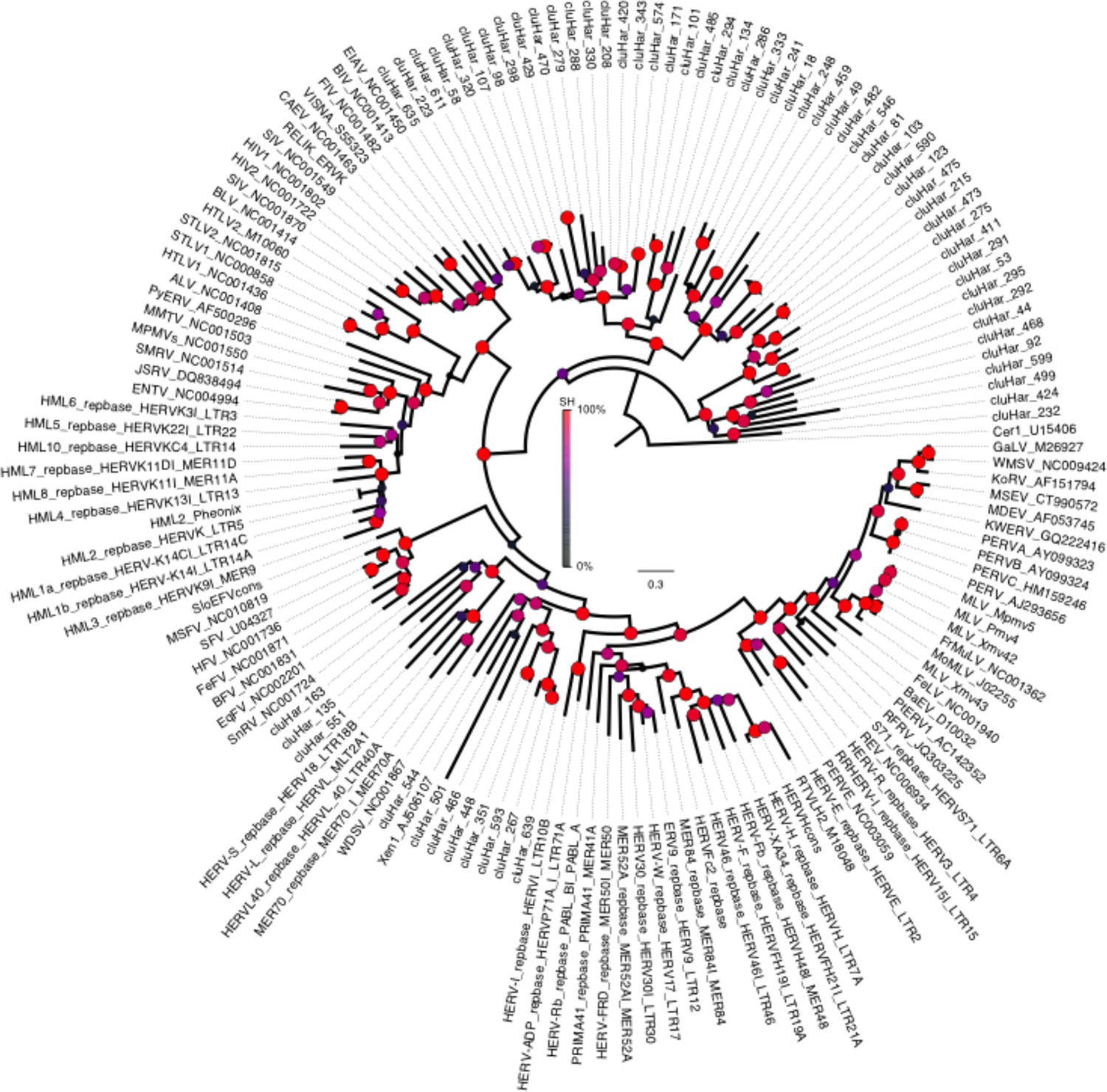
Phylogeny of endogenous retroviruses (ERVs).
Phylogeny of 62 Clupea harengus ERVs representing 150 detected ERVs, in relation to 92 reference sequences (Genbank and Repbase) rooted on the Cer1 retrotransposon. The phylogeny was constructed using FastTree2 (Price et al., 2010). Sequences and annotations for herring ERVs are presented in Supplementary file 2.
Figure 3 with 2 supplements

Genetic differentiation between Atlantic and Baltic herring.
(A) Manhattan plot of significance values testing for allele frequency differences between pools of herring from marine waters (Kattegat, Skagerrak, Atlantic Ocean) versus the brackish Baltic Sea. Lower panel, corresponding plot for scaffold 218 only; both P- and FST-values are shown. (B) Neighbor-joining phylogenetic tree based on all SNPs showing genetic differentiation in this comparison (p<10-10). (C) Comparison of allele frequencies in five strongly differentiated regions. The major allele in the AB1 sample (Atlantic Ocean) was used as reference at each SNP. Lower panel, neighbor-joining tree based on haplotypes formed by 128 differentiated SNPs from scaffold 218. (D) Heat map showing copy number variation partially overlapping the HCE gene. Orientation of transcription is marked with an arrow; the position of SNPs significant in the χ2 test is indicated by stars. Population samples and salinity at sampling locations are indicated to the right; abbreviations are explained in Table 2. (E) Strong genetic differentiation between Atlantic and Baltic herring in a region downstream of SLC12A3; statistical significance based on the χ2 test is indicated.
Figure 3—figure supplement 1
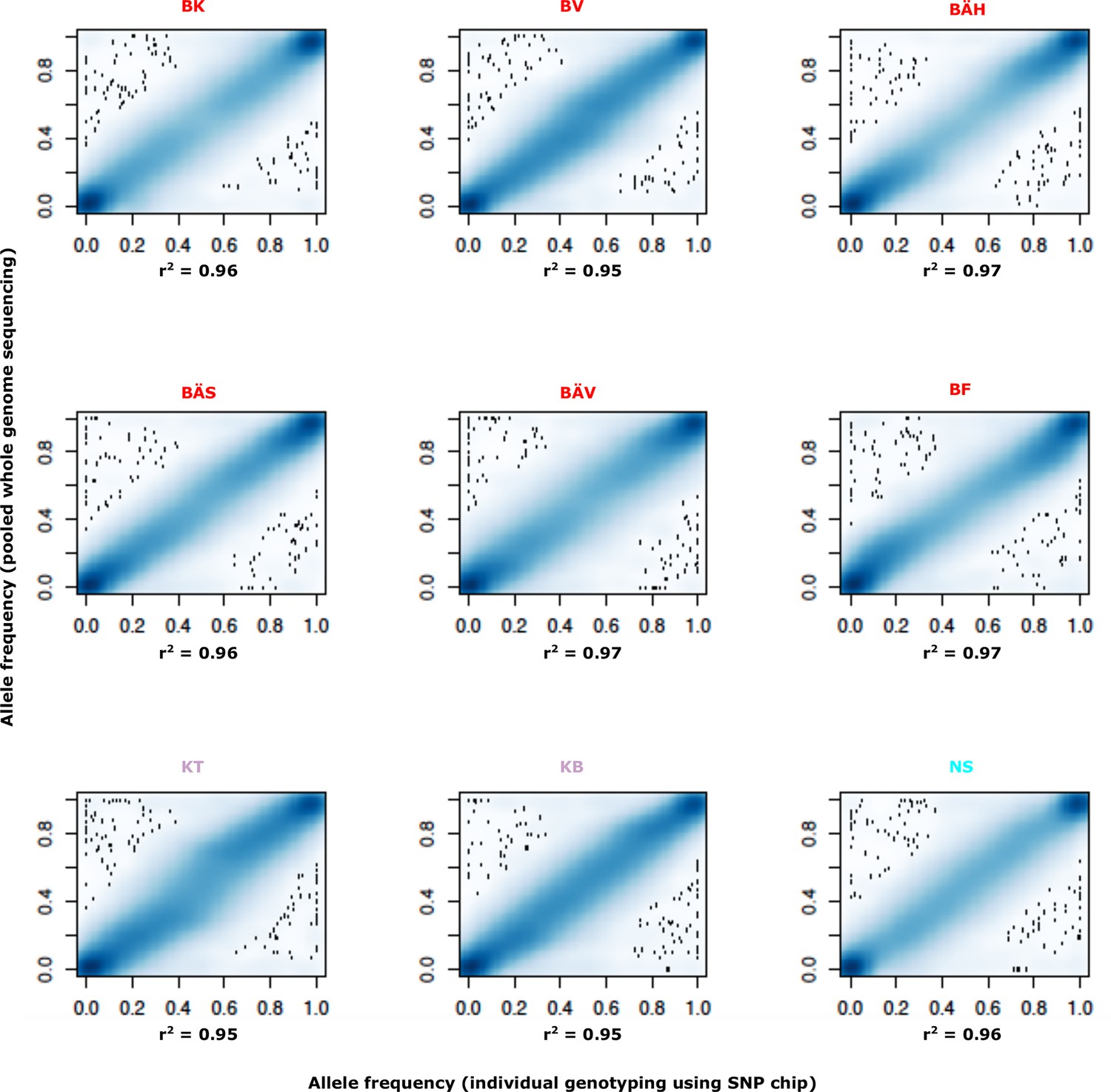
Comparison of allele frequencies estimated using pooled whole genome sequencing or by individual genotyping using a SNP chip.
Abbreviations for localities are given in Table 2.
Figure 3—figure supplement 2
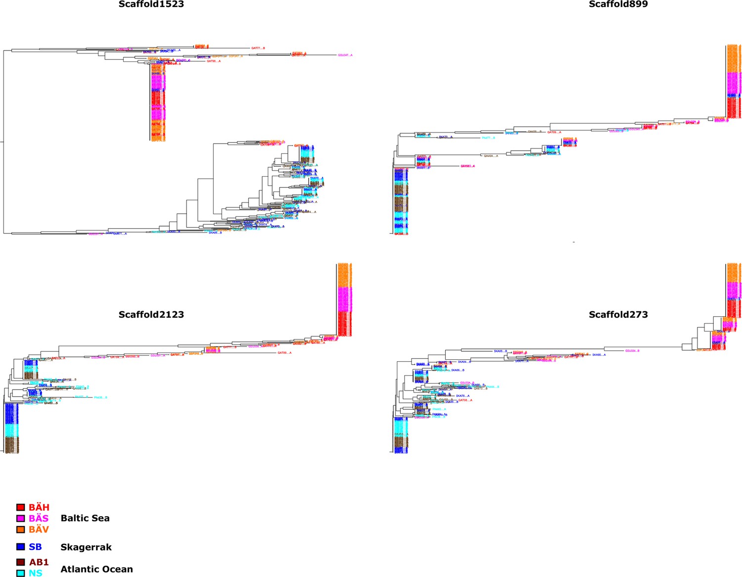
Additional neighbor-joining trees for the contrast Atlantic versus Baltic.
Trees based on individual SNP genotype data from four highly differentiated regions.
Figure 4 with 2 supplements
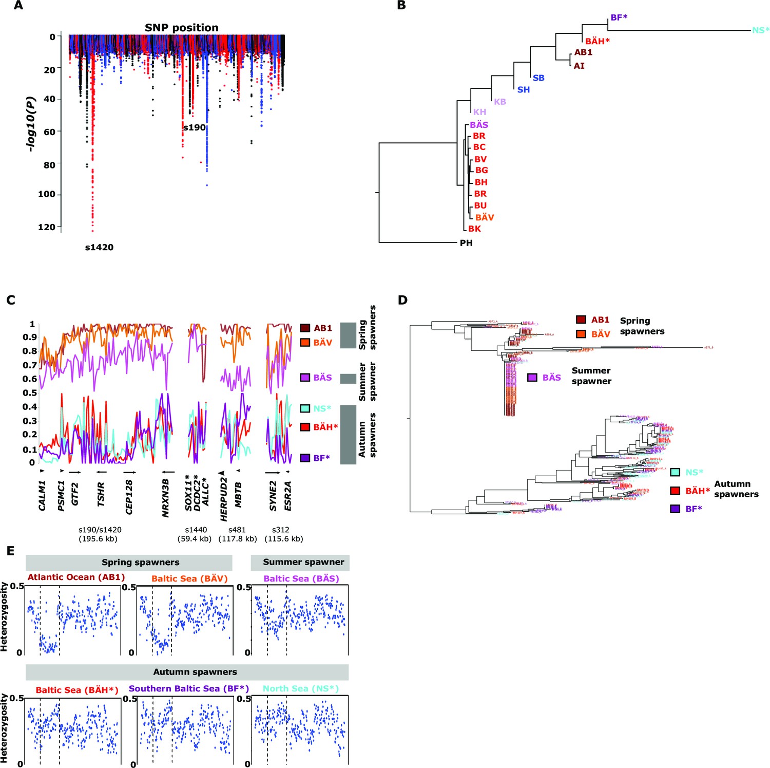
Genetic differentiation between spring- and autumn-spawning herring.
(A) Manhattan plot of significance values testing for allele frequency differences. (B) Neighbor-joining phylogenetic tree based on all SNPs showing genetic differentiation in this comparison (p<10-10). (C) Comparisons of allele frequencies in four strongly differentiated regions. The major allele in the AB1 sample (Atlantic Ocean) was set as reference at each SNP. Scaffolds 190 and 1420 have been merged in this plot since it was obvious that they were overlapping. *The signal in scaffold s1440 is present ~27 kb upstream of SOX11 and ~46 kb downstream of DCDC2/ALLC. (D) Neighbor-joining tree based on haplotypes formed by 70 differentiated SNPs from scaffold 190/1420; same populations as in Figure 4C. (E) Plot of average heterozygosity, per SNP in 5 kb windows, across scaffold 1420 indicating a selective sweep among spring-spawners in the region marked with vertical hatched lines. Autumn-spawning populations are marked by an asterisk.
Figure 4—figure supplement 1
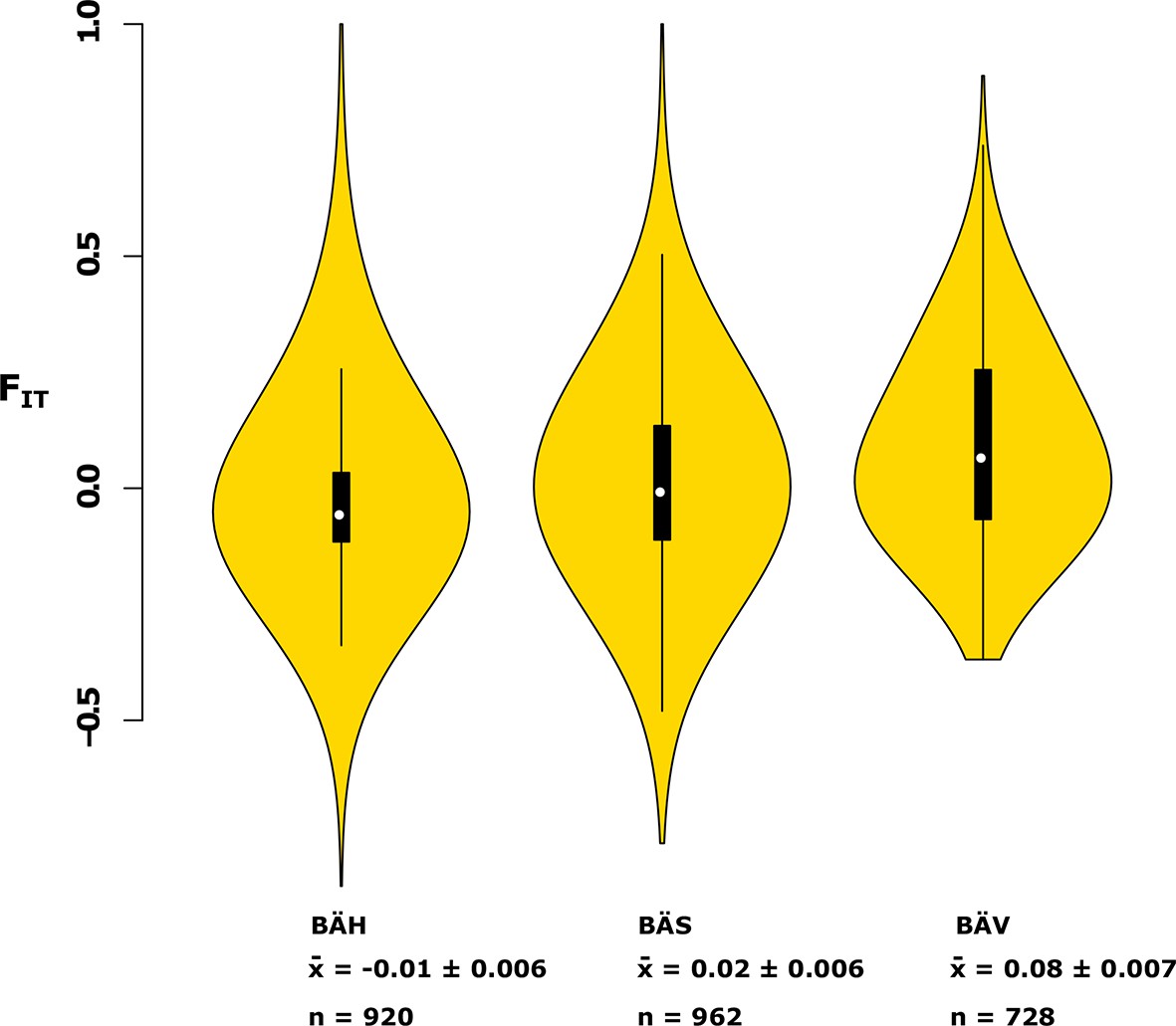
Analysis of deviations from Hardy-Weinberg equilibrium using the FIT statistic in spring- (BÄV), summer- (BÄS) and autumn- (BÄH) spawners from the same locality (Gävle).
The result is based on individual genotyping, using a SNP-chip, of 1500 SNPs that show strong genetic differentiation between spring- and autumn-spawners. The data are presented as a violin plot that shows a box plot in the middle and a rotated kernel density plot on each side. The central rectangle of the box plot spans the first to third quartiles of the distribution, and the ‘whiskers’ above and below the box show the maximum and minimum estimates. The line inside the rectangle shows the median. Mean FIT and its standard error is shown at the bottom; n represents the number of loci that was polymorphic in that particular population.
Figure 4—figure supplement 2
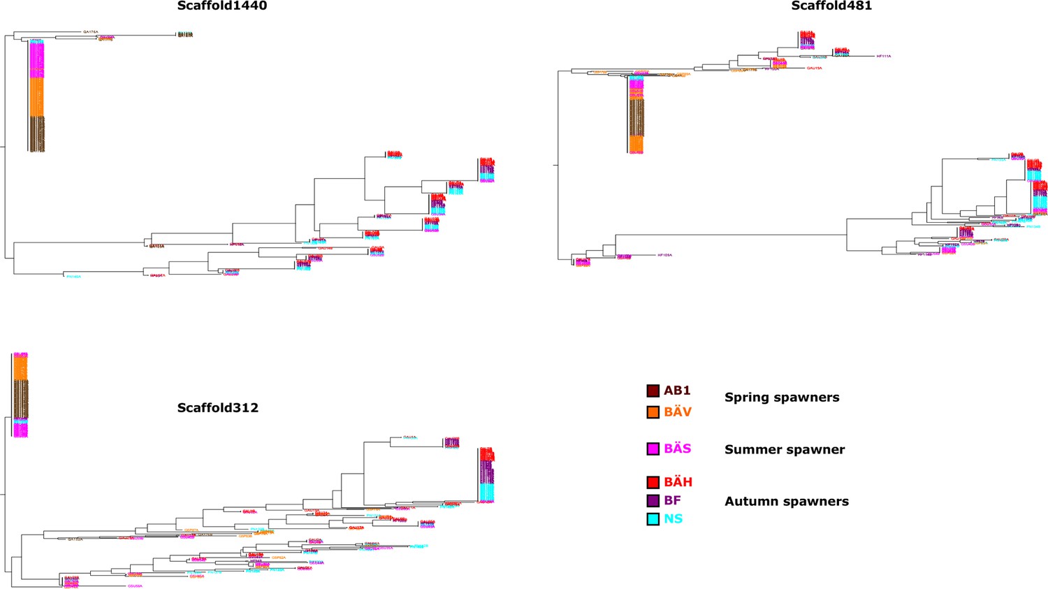
Additional neighbor-joining trees for the contrast between spring- and autumn spawning herring.
Trees based on individual SNP genotype data from three highly differentiated regions.
Figure 5

Nucleotide diversity within and between samples with different ecological adaptations as regards
(A) salinity and (B) spawning time. For each contrast 30 strongly differentiated regions of the genome and 30 control regions showing no significant differentiation were used. The nucleotide diversity within and between populations for the control regions was estimated around 0.3% consistent with the genome average whereas diversity in differentiated regions was significantly higher. BK=Baltic herring, Kalix; AB=Atlantic herring, Bergen; BÄH=autumn-spawning Baltic herring from Gävle; BÄV, spring-spawning Baltic herring from Gävle; see Table 1. The data are presented as box plots; the central rectangle spans the first to third quartiles of the distribution, and the ‘whiskers’ above and below the box show the maximum and minimum estimates. The line inside the rectangle shows the median.
Figure 6
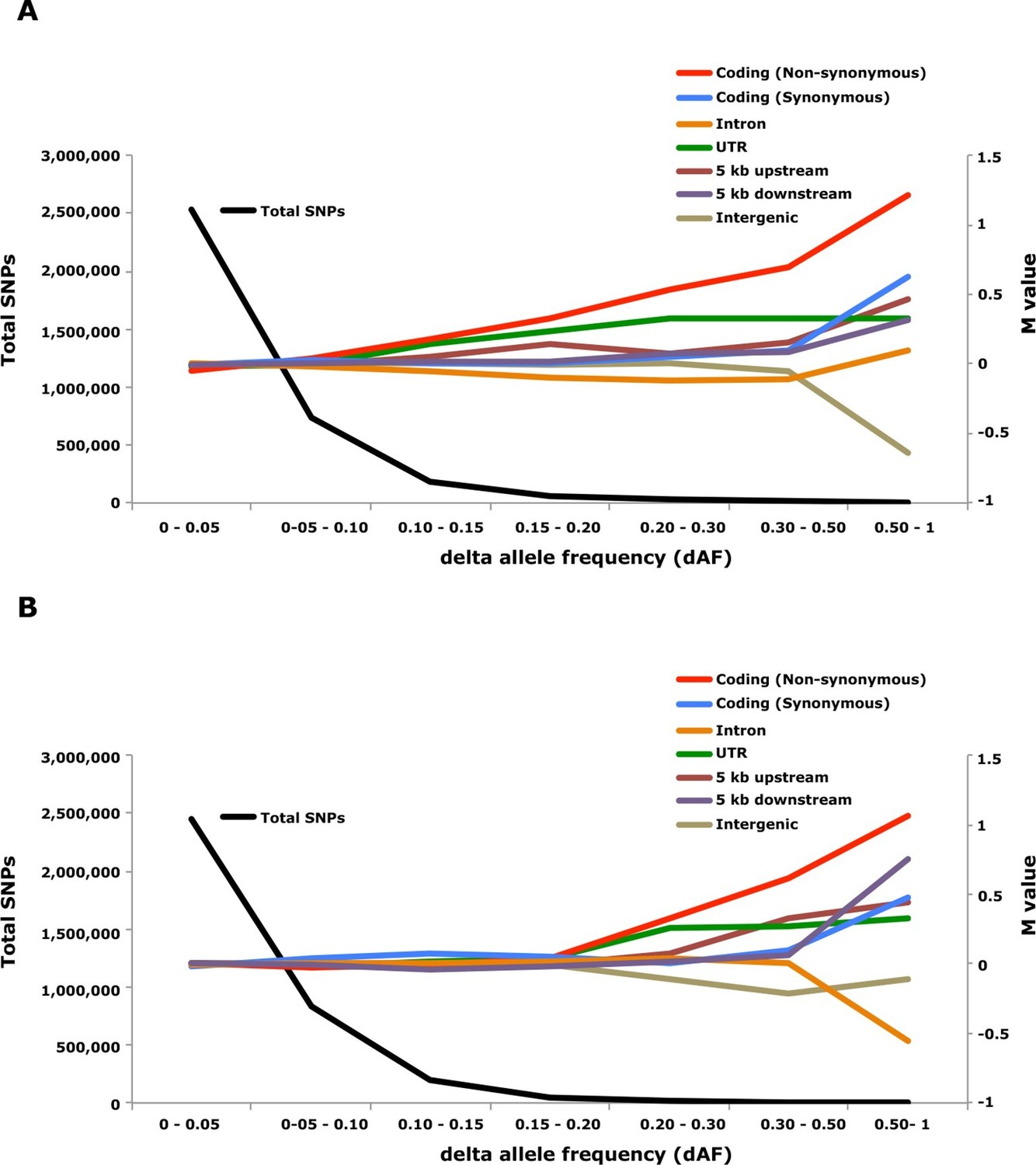
Analysis of delta allele frequency (dAF) for different categories of SNPs.
(A) dAF calculated for the contrast marine vs. brackish water. (B) dAF calculated for the contrast spring- vs. autumn-spawning. The black line represents the total number of SNPs in each dAF bin and coloured lines represent M values of different SNP types. M values were calculated by comparing the frequency of SNPs in a given annotation category in a specific bin with the corresponding frequency across all bins.
Tables
Table 1
Summary of the herring assembly compared to other sequenced fish genomes.
| Species | Herring (Clupea harengus) | Zebrafish (Danio rerio) | Cod (Gadus morhua) | Coelacanth (Latimeria chalumnae) | Stickleback (Gasteosteus aculeatus) |
|---|---|---|---|---|---|
| Estimated genome size (Mb) | 850 | 1,454a | 830b | 3,530c | 530d |
| Assembly size (Mb) | 808 | 1,412 | 753b | 2,861e | 463f |
| Contig N50 (kb) | 21.3 | 25.0 | 2.8 | 12.7 | 83.2 |
| Scaffold N50 (Mb) | 1.84 | 1.55 | 0.69 | 0.92 | 10.8 |
| Sequencing technologyg | I | S+I | R+I | I | S |
| Repeat content | 30.9 | 52.2 | 25.4 | 27.7 | 25.2 |
| %GC content | 44.1 | 36.7 | 45.4 | 43.0 | 44.6 |
| Heterozygosity | 1/309 | n.a. | 1/500 | 1/435 | 1/700 |
| Protein-coding gene count | 23,336 | 26,459 | 22,154 | 19,033 | 20,787 |
-
cGenome size calculated as pg x 0.978 × 10⁹ bp/pg; picogram values taken from Cimino and Bahr (1974)
-
gI=Illumina sequencing; S=Sanger sequencing; R=Roche 454 n.a.=not available
Table 2
Samples of herring used for whole genome resequencing.
| Localitya | Sample | n | Position | Salinity (‰) | Date (yy/mm/dd) | Spawning season | |
|---|---|---|---|---|---|---|---|
| Baltic Sea | |||||||
| Gulf of Bothnia (Kalix)b | BK | 47 | N 65°52’ | E 22°43’ | 3 | 800629 | spring |
| Bothnian Sea (Hudiksvall) | BU | 100 | N 61°45’ | E 17°30’ | 6 | 120419 | spring |
| Bothnian Sea (Gävle) | BÄV | 100 | N 60°43’ | E 17°18’ | 6 | 120507 | spring |
| Bothnian Sea (Gävle) | BÄS | 100 | N 60°43’ | E 17°18’ | 6 | 120718 | summer |
| Bothnian Sea (Gävle) | BÄH | 100 | N 60°44’ | E 17°35’ | 6 | 120904 | autumn |
| Bothnian Sea (Hästskär)c | BH | 50 | N 60°35’ | E 17°48’ | 6 | 130522 | spring |
| Central Baltic Sea (Vaxholm)b | BV | 50 | N 59°26’ | E 18°18’ | 6 | 790827 | spring |
| Central Baltic Sea (Gamleby)b | BG | 49 | N 57°50’ | E 16°27’ | 7 | 790820 | spring |
| Central Baltic Sea (Kalmar) | BR | 100 | N 57°39’ | E 17°07’ | 7 | 120509 | spring |
| Central Baltic Sea (Karlskrona) | BA | 100 | N 56°10’ | E 15°33’ | 7 | 120530 | spring |
| Central Baltic Sea | BC | 100 | N 55°24’ | E 15°51’ | 8 | 111018 | unknown |
| Southern Baltic Sea (Fehmarn)b | BF | 50 | N 54°50’ | E 11°30’ | 12 | 790923 | autumn |
| Kattegat, Skagerrak, North Sea, Atlantic Ocean | |||||||
| Kattegat (Träslövsläge)b | KT | 50 | N 57°03’ | E 12°11’ | 20 | 781023 | unknown |
| Kattegat (Björköfjorden) | KB | 100 | N 57°43’ | E 11°42’ | 23 | 120312 | spring |
| Skagerrak (Brofjorden) | SB | 100 | N 58°19’ | E 11°21’ | 25 | 120320 | spring |
| Skagerrak (Hamburgsund)b | SH | 49 | N 58°30’ | E 11°13’ | 25 | 790319 | spring |
| North Seab | NS | 49 | N 58°06’ | E 06°10’ | 35 | 790805 | autumn |
| Atlantic Ocean (Bergen)b | AB1 | 49 | N 64°52’ | E 10°15’ | 35 | 800207 | spring |
| Atlantic Ocean (Bergen)c | AB2 | 8 | N 60°35’ | E 05°00’ | 33 | 130522 | spring |
| Atlantic Ocean (Höfn) | AI | 100 | N 65°49’ | W 12°58’ | 35 | 110915 | spring |
| Pacific Ocean | |||||||
| Strait of Georgia (Vancouver) | PH | 50 | - | - | 35 | 121124 | - |
-
aPlaces where the sample was landed (if known) are given in parenthesis
-
bSamples from previous study (Lamichhaney et al., 2012)
-
cEight Baltic herring from the BH sample and eight Atlantic herring from the AB2 sample were used for individual sequencing n=number of fish
Additional files
-
Supplementary file 1
(A) Summary of sequencing data used to generate the herring genome assembly. (B) Statistics of the herring genome assembly developed using SOAPdenovo. v1.0 to v1.4 refer to different versions of the assembly. Full description of the assembly process is provided within the Methods section. (C) Statistics for genome completeness based on 248 annotated core eukaryotic genes (CEGs) by CEGMA. (D) Statistics for the annotated protein-coding genes. (E) Statistics for annotated repeats. (F) Comparison of indels discovered using Illumina short reads or synthetic long reads (SLRs) in the reference herring genome.
- https://doi.org/10.7554/eLife.12081.021
-
Supplementary file 2
Endogenous retroviruses detected with RetroTector.
- https://doi.org/10.7554/eLife.12081.022
-
Supplementary file 3
(A) List of loci showing strong genetic differentiation between Atlantic and Baltic herring (p<10-10). (B) List of structural changes associated with genetic differentiation between Atlantic and Baltic herring. (C) List of loci showing strong genetic differentiation between spring- and autumn-spawning herring (p<10-10). (D) List of structural changes associated with genetic differentiation between spring- and autumn-spawning herring. (E) Genomic distributions of different categories of SNPs in different delta allele frequency (dAF) bins. Only SNPs called in all populations that had confident annotations were used in this analysis. (F) Non-synonymous substitutions showing strong genetic differentiation, delta allele frequency (dAF) >0.5. (G) Analysis of delta allele frequencies (dAF) for SNPs in 5'UTR and 3'UTR. Only SNPs called in all populations that had confident annotations were used in this analysis. (H) Analysis of delta allele frequencies (dAF) for SNPs within the 5 kb region upstream of start of transcription.
- https://doi.org/10.7554/eLife.12081.023
Download links
A two-part list of links to download the article, or parts of the article, in various formats.
Downloads (link to download the article as PDF)
Open citations (links to open the citations from this article in various online reference manager services)
Cite this article (links to download the citations from this article in formats compatible with various reference manager tools)
The genetic basis for ecological adaptation of the Atlantic herring revealed by genome sequencing
eLife 5:e12081.
https://doi.org/10.7554/eLife.12081


