The hierarchical organization of the lateral prefrontal cortex
- University of California, United States
Figures
Figure 1 with 1 supplement
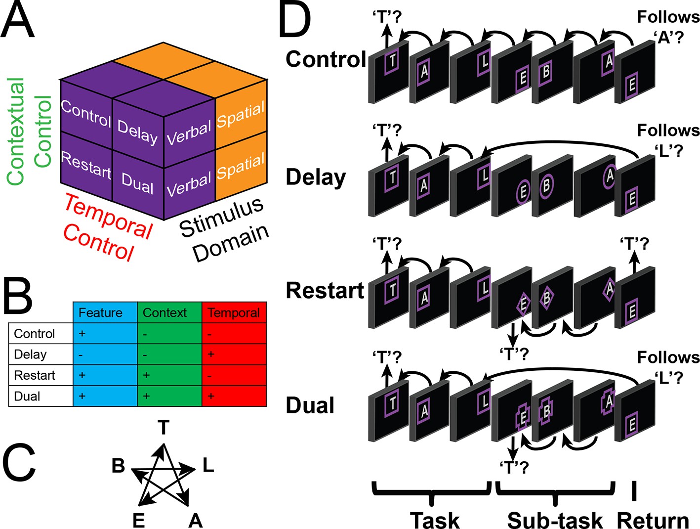
Experimental design.
(A) The design orthogonally manipulated factors of Stimulus Domain (verbal, spatial) and two forms of cognitive control: Contextual Control (low – Control, Delay; high – Restart, Dual) and Temporal Control (low – Control, Restart; high – Delay, Dual). These factors were fully crossed in a 2 x 2 x 2 design. (B) Cognitive control processes engaged by condition. (C) The basic task required participants to judge whether a stimulus followed the previous stimulus in a sequence. The sequence in the verbal task was the order of the letters in the word 'tablet.' The sequence in the spatial task was a trace of the points of a star. The start of each sequence began with a decision regarding whether the currently viewed stimulus is the start of the sequence (e.g. ‘t’ in the verbal task). (D) Factors were blocked with each block containing a basic task phase, a sub-task phase, a return trial, and a second basic task phase (not depicted), for all but the Control blocks. Control blocks consisted only of the basic task phase extended to match the other conditions in duration. Colored frames indicated whether letters or locations were relevant for the block (verbal – purple; spatial – orange in this example; verbal condition depicted). The basic task was cued by square frames. Other frames cued the different sub-task conditions. In the Delay condition (circle frames), participants held in mind the place in the sequence across a distractor-filled delay. In the Restart condition (diamond frames), participants started a new sequence. In the Dual condition (cross frames), participants simultaneously started a new sequence, and maintained the place in the previous sequence.
Figure 1—figure supplement 1
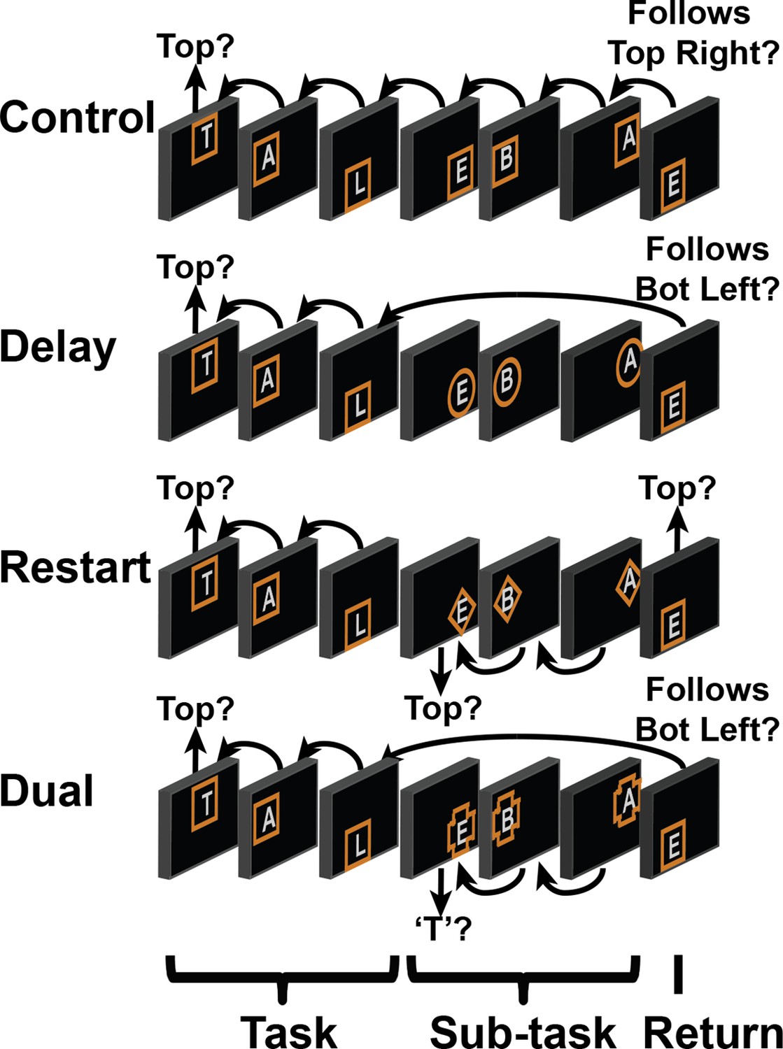
Spatial task.
Example blocks of the spatial task wherein participants decided whether the stimulus followed the preceding stimulus in a star trace (Figure 1C). Details are otherwise identical to Figure 1.
Figure 2

Behavioral results.
Reaction times (top) and error-rates (bottom) as a function of condition in the sub-task (left) and return trials (right). Comparisons reflect Bonferroni corrected tests against the Control condition. *pcorrected<0.05, **pcorrected<0.005; ***pcorrected<0.0005.
Figure 3 with 5 supplements

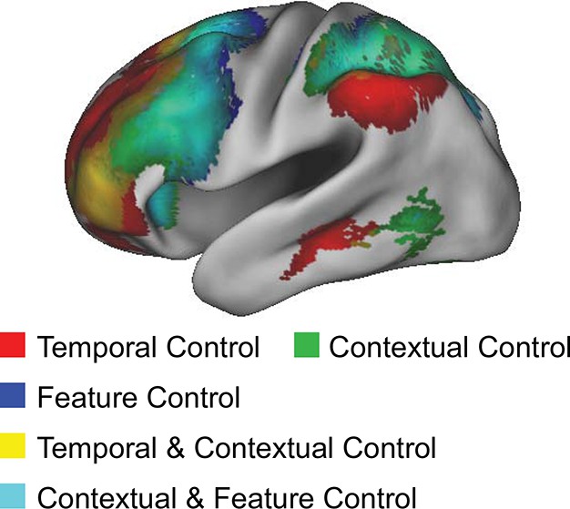
Univariate whole-brain results.
Temporal demands of cognitive control produced a gradient of activation along the rostral/caudal axis of the LPFC. Temporal Control activated the rostral LPFC (red), Contextual Control the mid LPFC (green), and the interaction relating to Feature Control the caudal LPFC (blue). All results are corrected for multiple comparisons. Darker colors: p<10–3; Brighter colors: p<10–8 (Temporal Control, Feature Control) or p<10–12 (Contextual Control) to better visualize peaks.
-
Figure 3—source data 1
Statistical parametric maps of the univariate whole-brain results.
Maps contain t-statistics and have been thresholded to correct for multiple comparisons as detailed in the Materials and methods.
- https://doi.org/10.7554/eLife.12112.007
Figure 3—figure supplement 1
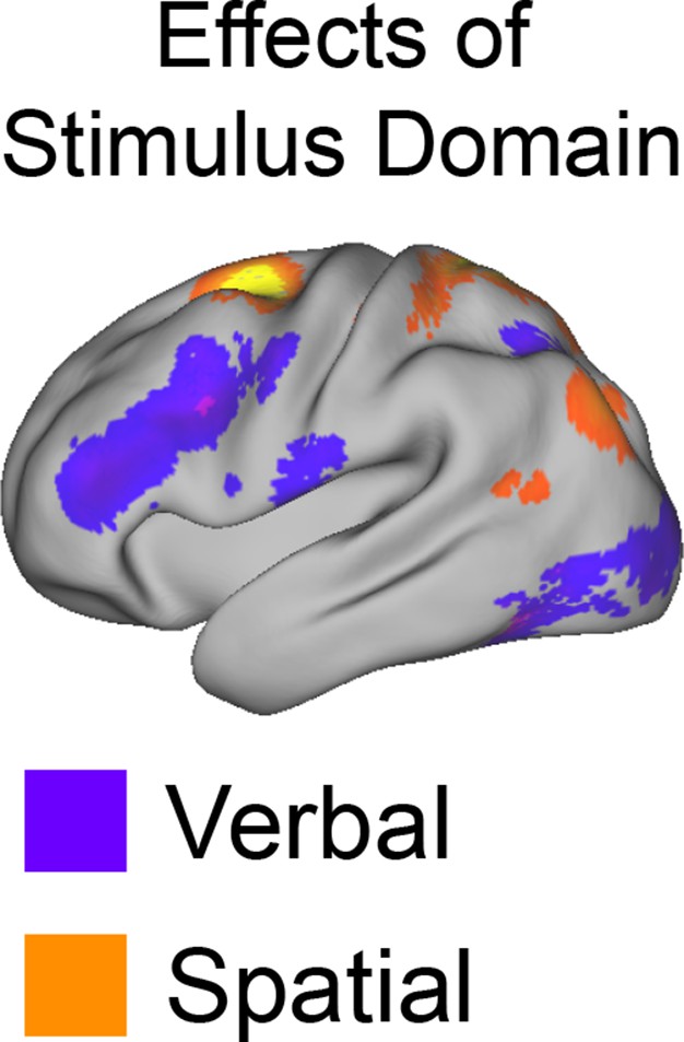
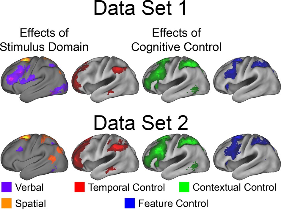
Univariate whole-brain results of Stimulus Domain.
Demands on Stimulus Domain produced differences along the dorsal/ventral axis of the LPFC. Effects of verbal processing (verbal > spatial; purple) were observed in the ventral LPFC, while effects of spatial processing (spatial > verbal; orange) were observed in the dorsal LPFC.
Figure 3—figure supplement 2
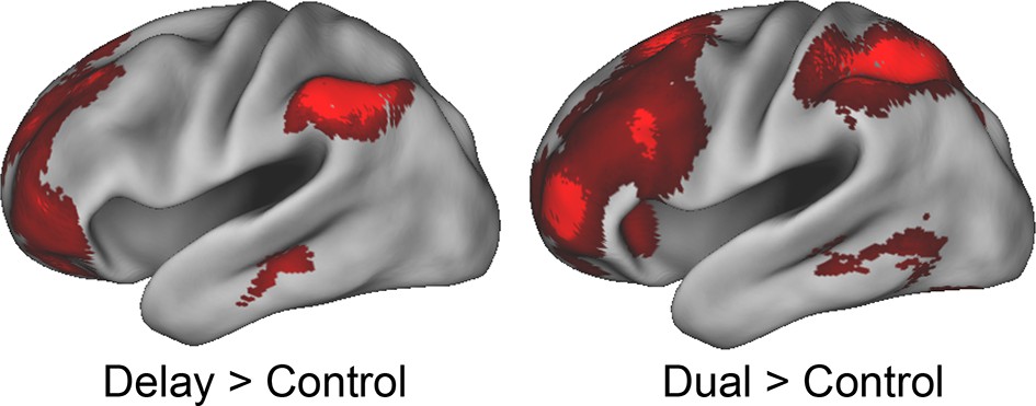
Effects of delay and dual.
Despite being associated with the fastest reaction times and lowest error-rates, the Delay condition demonstrated activation in the rostral-most areas of the LPFC. These results indicate that the activations do not reflect difficulty, time-on-task, or attention. Conversely, the Dual condition demonstrated the slowest reactions times and highest error-rates, and produced convergent activations in the rostral-most areas of the LPFC. These results indicate that the activations do not reflect ease or 'default' activity.
Figure 3—figure supplement 3
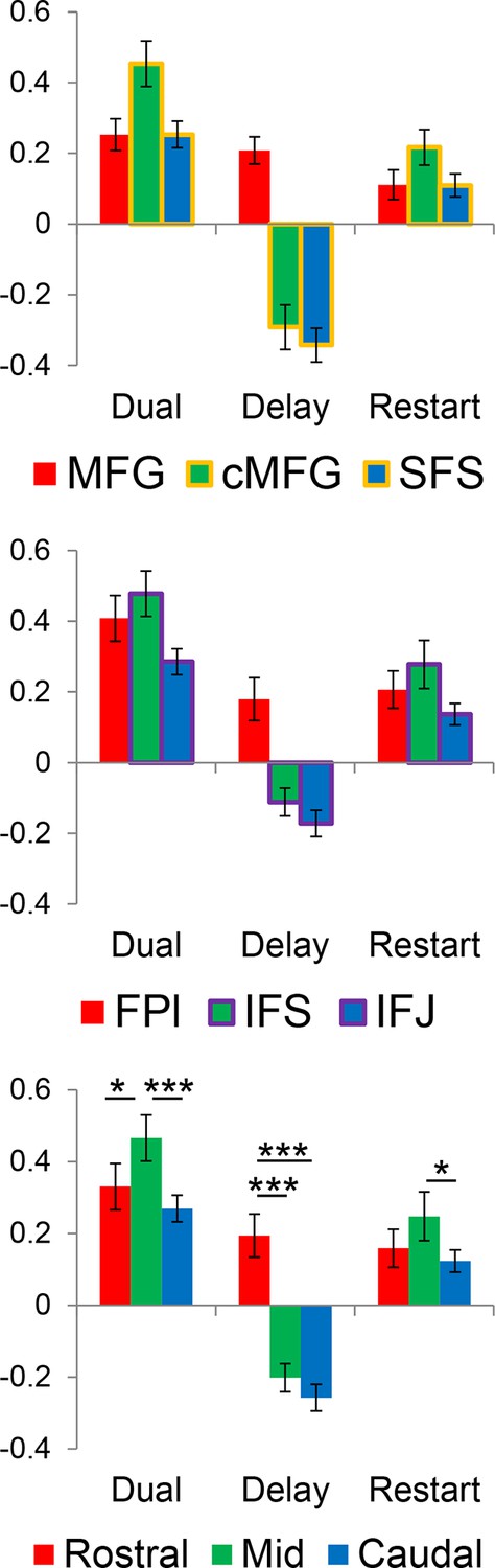
Activation magnitudes within regions-of-interest.
Bars represent contrasts of each cognitive control condition against the Control condition, collapsing across Stimulus Domain. Data were split to provide unbiased estimates of activation (see Materials and methods). Given the similar activation patterns between dorsal (MFG, cMFG, SFS) and ventral (FPl, IFS, IFJ) areas, data were averaged by rostral/caudal zone collapsing across the dorsal/ventral axis for statistical tests. *pcorrected<0.05; ***pcorrected<0.0005.
Figure 3—figure supplement 4
Gradient visualization.
Contrasts of cognitive control overlaid to visualize the gradient and extent of LPFC coverage.
Figure 3—figure supplement 5
Univariate whole-brain robustness.
Data were split into two data sets through an alternating runs procedure. Whole-brain univariate contrasts were repeated for each data set and are depicted above. Details are otherwise identical to Figure 3 in the main text.
Figure 4 with 1 supplement
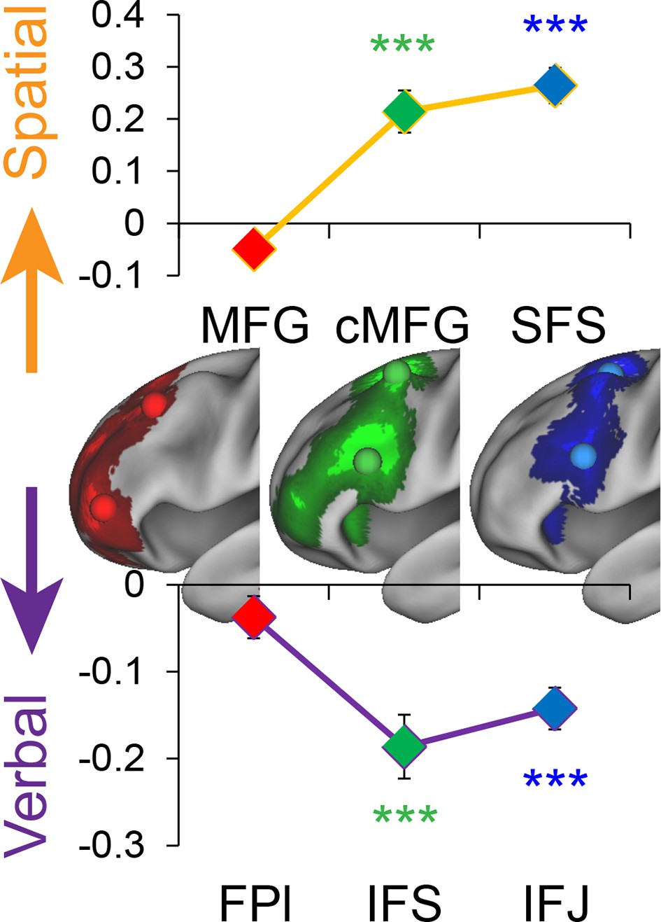
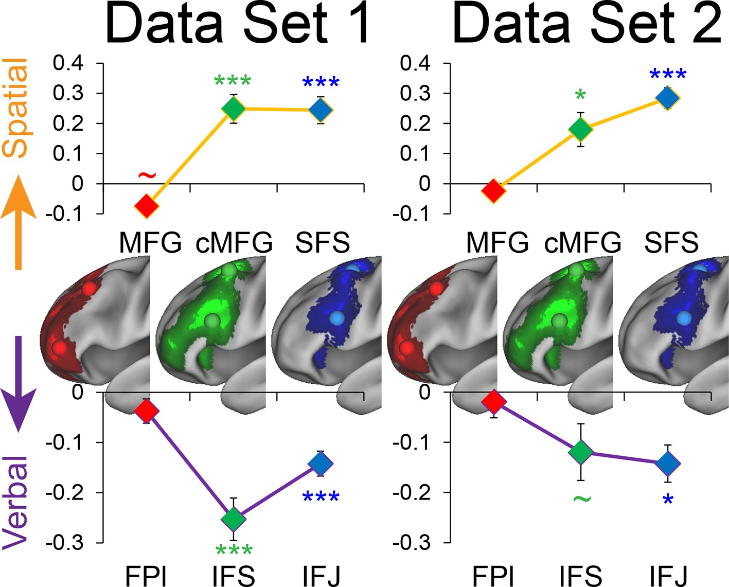
Stimulus domain-sensitivity along the rostral/caudal axis.
Regions defined by peak effects of Temporal Control (red), Contextual Control (green), and Feature Control (blue). Points reflect the contrast estimates for spatial – verbal such that positive values represent spatial sensitivity and negative values represent verbal sensitivity. Stimulus domain-sensitivity was observed in caudal and mid, but not rostral areas of the LPFC. ***pcorrected<0.0005.
Figure 4—figure supplement 1
Stimulus domain-sensitivity along the rostral/caudal axis robustness.
Data were split into two data sets through an alternating runs procedure. Region-of-interest analyses were repeated for each data set and are depicted above. Details are otherwise identical to Figure 4 in the main text. ~puncorrected<0.05; *pcorrected<0.05; ***pcorrected<0.0005.
Figure 5 with 1 supplement
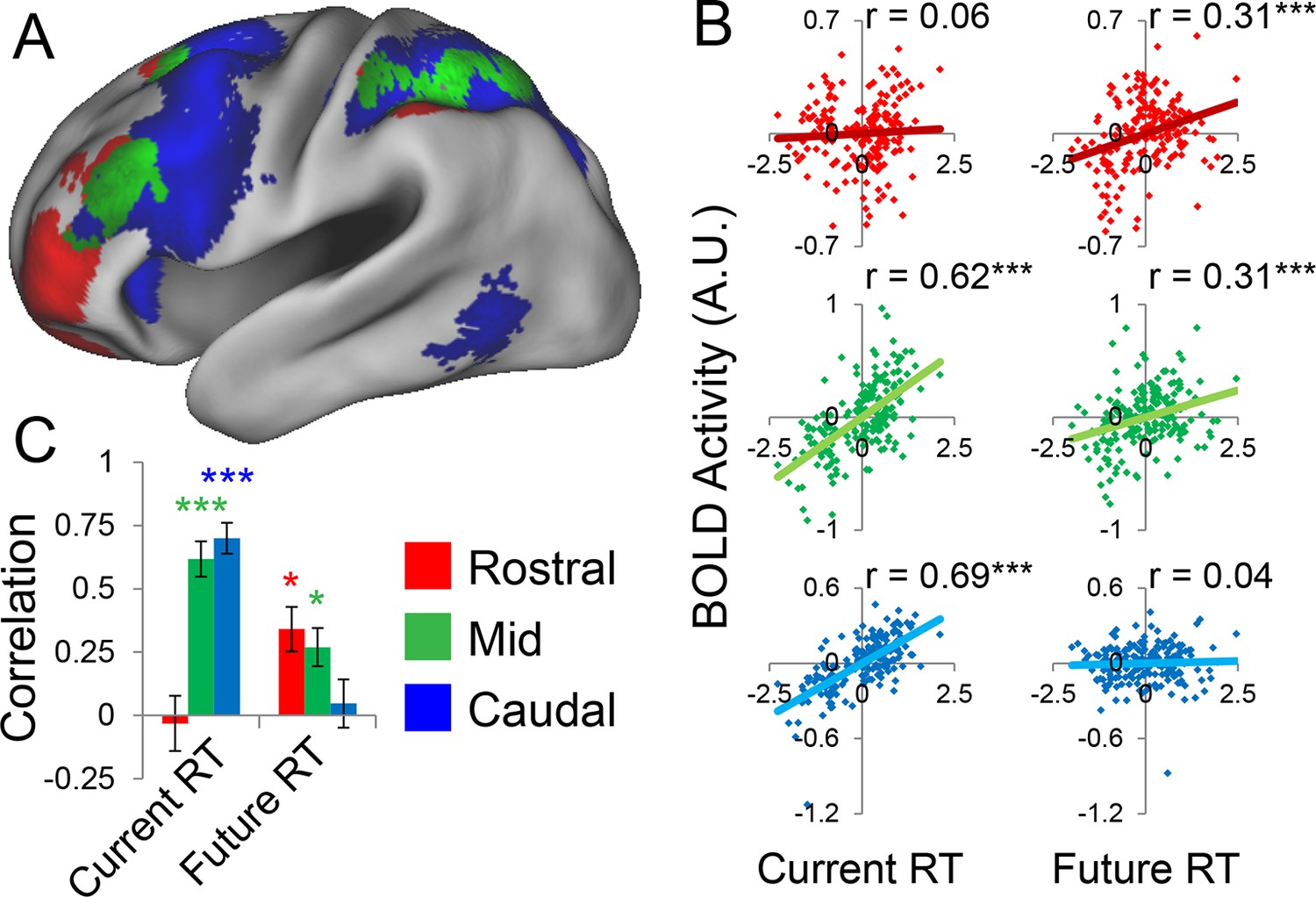
Temporal activation-behavior relationships.
Correlations between activation and reaction time (RT). Current RT corresponds to sub-task trials while future RT corresponds to return trials. RT measures have been normalized within-subject across the 8 conditions of interest. (A) Voxel-wise regression of Current and Future RT onto activations for the 8 conditions of interest across subjects. Individual subject terms have been regressed out. Red: significant correlations with Future RT only; Blue: significant correlations with Current RT only; Green: both. (B) Partial correlations between activation and RT for the 8 conditions of interest for all subjects. Individual subject terms have been regressed out. Red: rostral LPFC; Green: mid LPFC; Blue: caudal LPFC. (C) Average partial correlation computed separately for each subject (summary-statistic approach). *pcorrected<0.05; ***pcorrected<0.0005.
-
Figure 5—source data 1
Statistical parametric maps of the activation-behavior correlations.
Maps contain r-values and have been thresholded to correct for multiple comparisons as detailed in the Materials and methods.
- https://doi.org/10.7554/eLife.12112.016
Figure 5—figure supplement 1
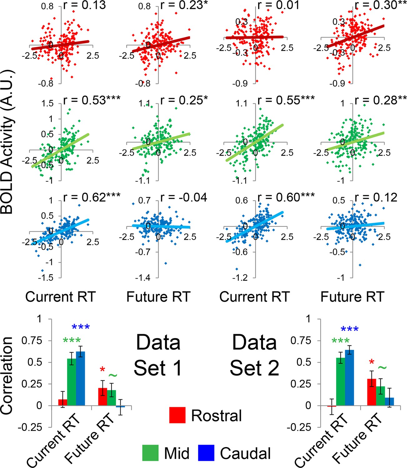
Temporal activation-behavior relationships robustness.
Data were split into two data sets through an alternating runs procedure. Correlations were computed for each dataset in the same way as depicted in Figure 5 of the main text. ~puncorrected<0.05; *pcorrected<0.05; **pcorrected<0.005; ***pcorrected<0.0005.
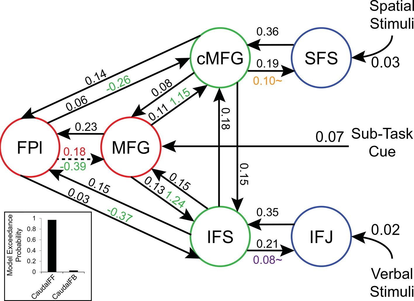
Figure 6 with 5 supplements
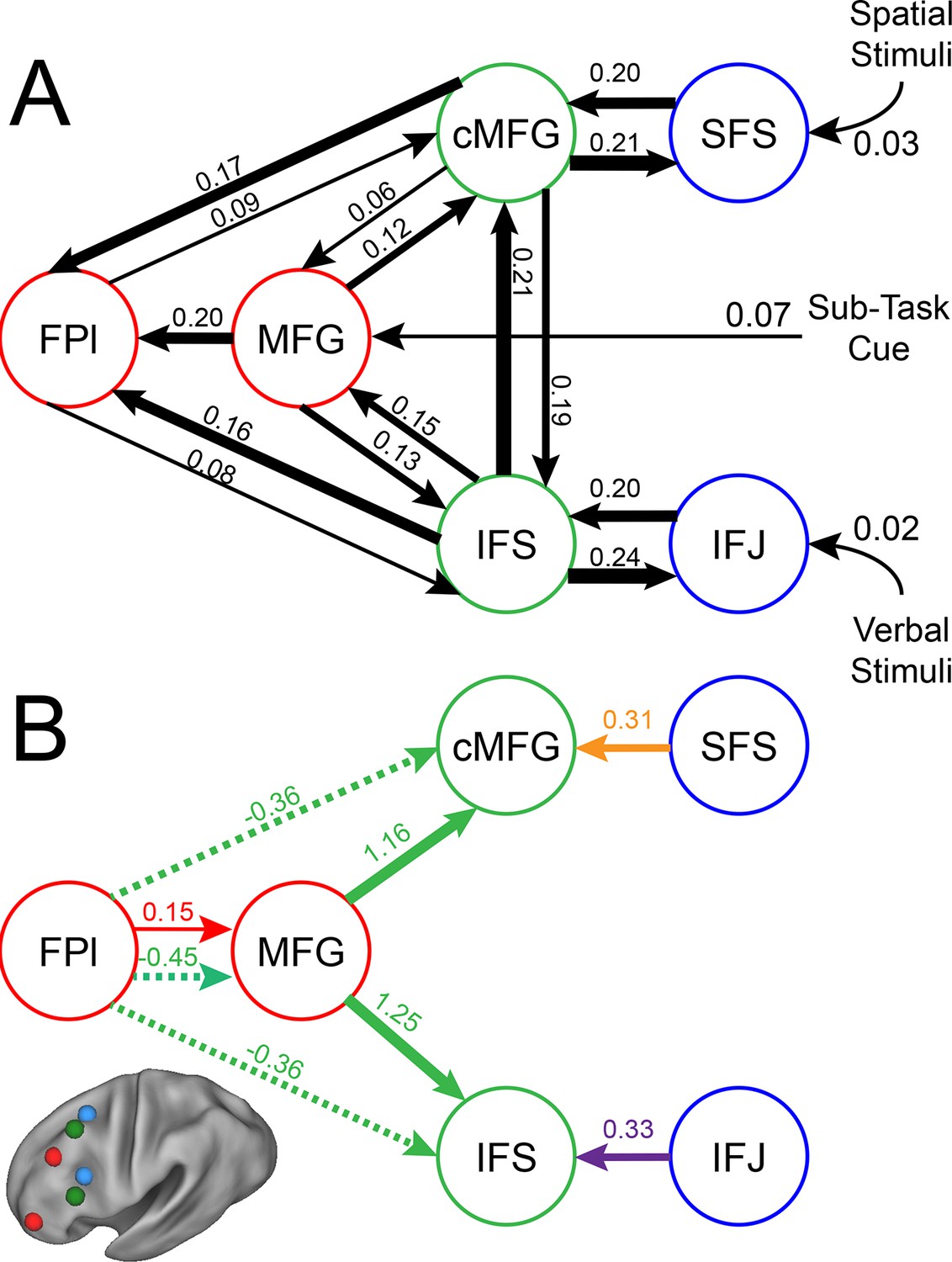
LPFC dynamic causal model.
Interactions within the LPFC were modeled using dynamic causal modeling. Bayesian model selection indicated that the depicted model was the best model of the dynamics among the models tested. Arrows indicate direction of influence, numbers and line widths indicate the strength of influence, and dashed arrows indicated inhibitory influences. (A) Fixed connectivity and inputs depicted in black. (B) Modulations of connectivity by Spatial Stimulus Domain (orange), Verbal Stimulus Domain (purple), Contextual Control (green), and Temporal Control (red) demands depicted in colors. Stimulus Domain demands produced feedforward influences from caudal areas (blue) to mid areas (green). Cognitive control demands produced feedback influences from rostral (red) to mid areas (green). All depicted parameters are significant after correction using false-discovery rate.
Figure 6—figure supplement 1
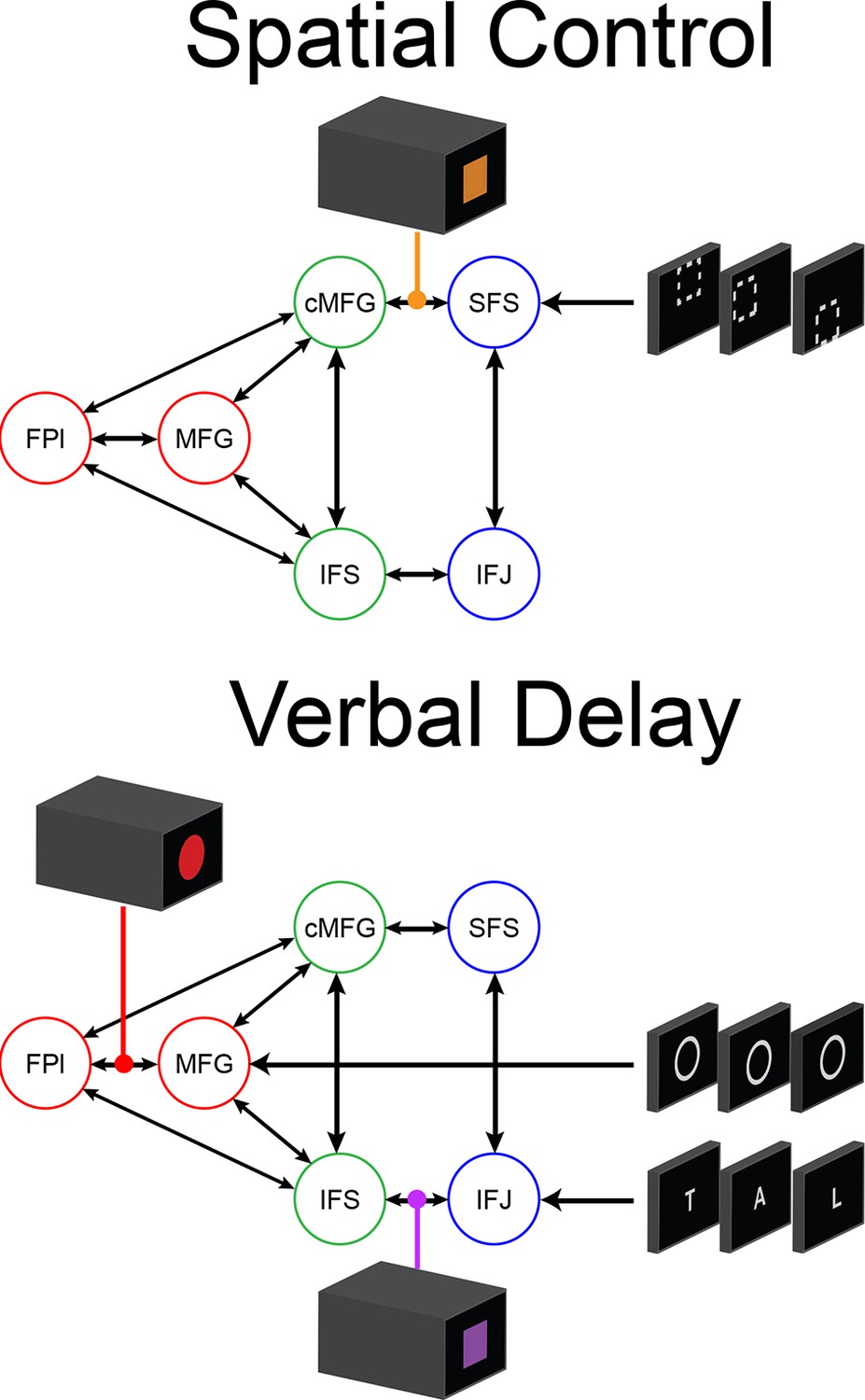
Depiction of dynamic causal modeling.
Tiles represent transient stimuli while blocks represent sustained modulations. For simplicity, all modulations are depicted as bidirectional. Top: an example of a Spatial Control block. Spatial location stimuli are modeled as inputs into SFS. Additional tonic influences of Spatial processing are modeled as modulators of connectivity between areas SFS and cMFG. Bottom: an example of a Verbal Delay block. Verbal letter stimuli are modeled as inputs to IFJ, while the task cues signaling the Delay sub-task are modeled as inputs to MFG. Tonic influences of Verbal processing are modeled as modulators of connectivity between IFJ and IFS, while influences of Temporal Control are modeled as modulators of connectivity between FPl and MFG.
Figure 6—figure supplement 2

LPFC dynamic causal model robustness.
Data were split into two data sets through an alternating runs procedure. Black numbers indicate input and fixed connectivity parameter estimates Colored numbers indicated modulations by Spatial Stimulus Domain (orange), Verbal Stimulus Domain (purple), Contextual Control (green), and Temporal Control (red). Of the 29 parameters estimated, only a single parameter was significant in one dataset and not the other.
Figure 6—figure supplement 3
Path coefficients in a rostral-to-caudal model.
Inference on parameters was performed on an alternative model of LPFC organization wherein content demands produced feedback modulations from mid areas to caudal areas. Notably, this is a strict rostral-to-caudal hierarchical model of modulations. Inset: Model comparison demonstrating the inferiority of this model (CaudalFB) to the chosen model depicted in Figure 6 (CaudalFF). These data stress the importance of explicit model comparison prior to inference on parameters. Details otherwise identical to Figure 6 – supplement 1. ~q<0.05, one-tailed.
Figure 6—figure supplement 4
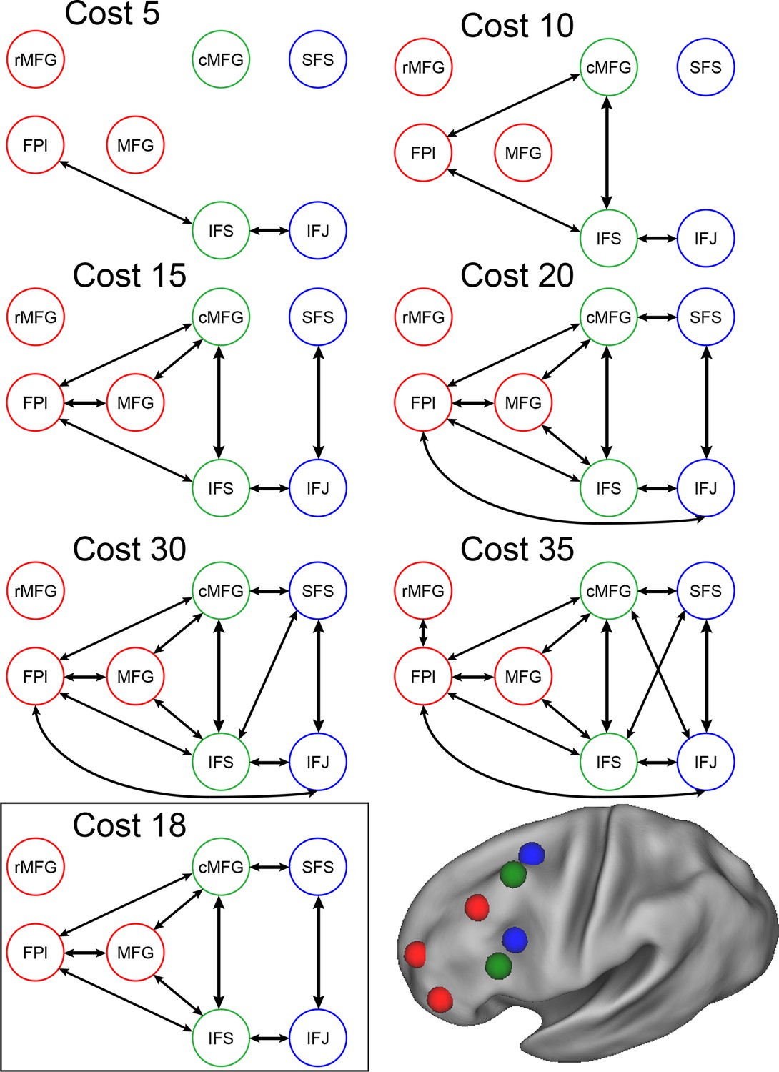
Connectivity as a function of cost.
Examples of connectivity profiles at different costs are depicted. The chosen connectivity profile was at cost 18, falling in the middle of the sampling range. rMFG was disconnected from the rest of the network at all but the highest cost levels and was therefore excluded from various analyses.
Figure 6—figure supplement 5
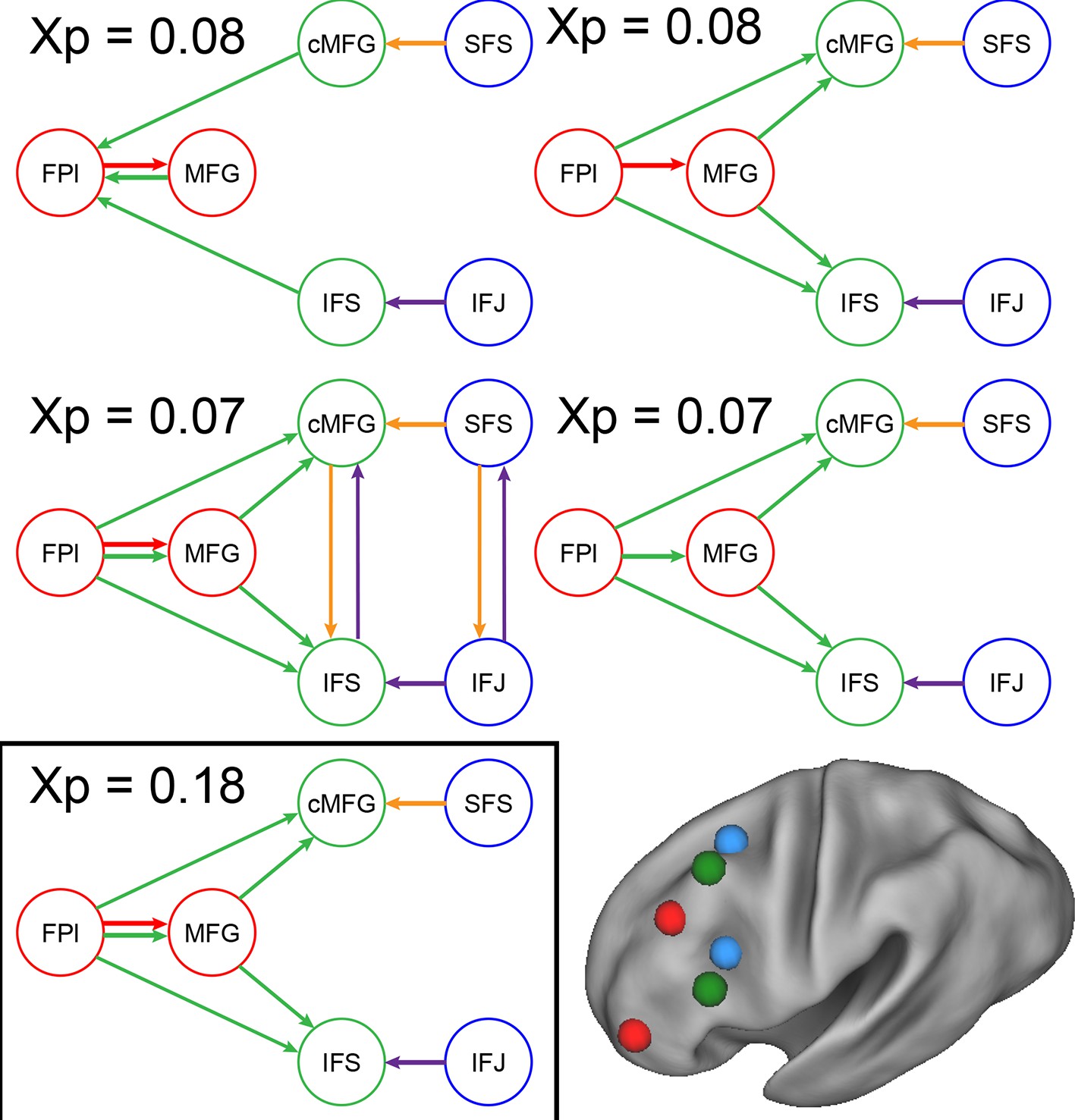
Model comparison.
Modulatory parameter structure for the winning (bottom left) and closest competitor models. The depicted models are the only models with exceedance probabilities (Xp) greater than 0.05, among the 99 models examined. The closest competitors all closely resembled the winning model. Red arrows – modulation by Temporal Control; green arrows – modulation by Contextual Control; orange arrows – modulation by Spatial Stimulus Domain; purple arrows – modulation by Verbal Stimulus Domain.
Figure 7 with 2 supplements

Hierarchical structural dependencies.
Based on fixed connectivity of the model depicted in Figure 6A, hierarchical strength was calculated as the difference between inward and outward projections along the rostral/caudal axis. Hierarchical strength rose monotonically from caudal to mid areas, but fell precipitously at the rostral most portion of the network. **pcorrected<0.005; ***pcorrected<0.0005.
Figure 7—figure supplement 1

Hierarchical structural dependency robustness.
Data were split into two data sets through an alternating runs procedure. Details are otherwise identical to Figure 7 in the main text.
Figure 7—figure supplement 2

Average and total connectivity strength.
(A) Average connectivity strength reflects the mean of rostral/caudal fixed connectivity for each region. (B) Total connectivity strength reflects the sum of rostral/caudal fixed connectivity. Both of these patterns were substantially different than the inverted-U pattern observed in hierarchical strength.
Figure 8 with 3 supplements
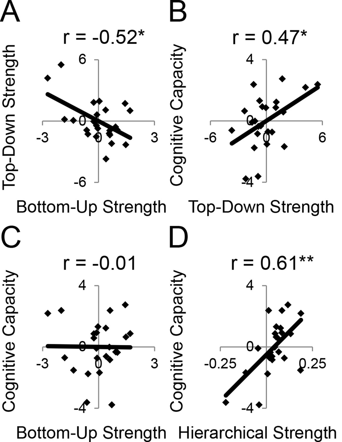
LPFC dynamics and higher-level cognitive ability.
Neural metrics were based on modeled estimates of effective connectivity and their modulations (Figure 6). Metrics reflecting top-down LPFC modulations by cognitive control demands (top-down strength), and metrics reflecting bottom-up LPFC modulations by Stimulus Domain demands (bottom-up strength) were combined, respectively. (A) Top-down and bottom-up strength were anti-correlated. (B) Top-down strength predicted trait-measured higher-level cognitive capacity. (C) By contrast, bottom-up strength did not correlate with higher-level cognitive capacity. (D) Hierarchical strength reflected the degree to which mid LPFC showed greater outward than inward fixed connectivity. This metric was also positively related to higher-level cognitive capacity. *p<0.05; **p<0.005.
Figure 8—figure supplement 1
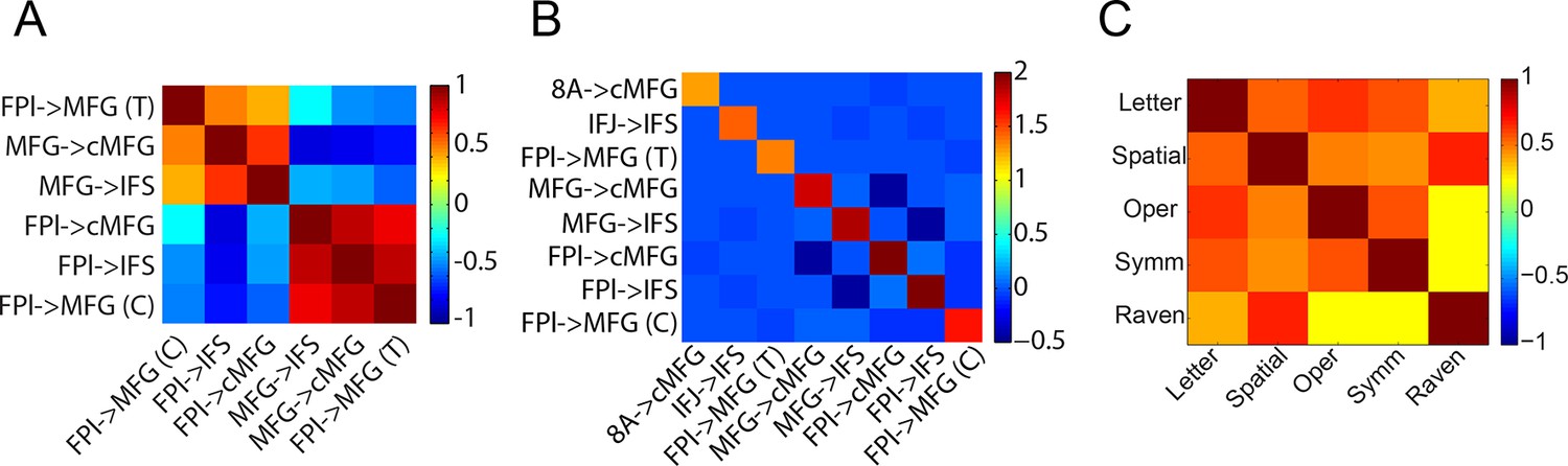
Model and trait correlations and covariances.
(A) Correlations between top-down parameters. Individual differences in the magnitude of top-down modulations tended to be correlated. The negative correlations reflect anti-correlation between parameters that were positive and negative, thereby reflecting a positive co-variation in magnitude. (B) Model covariance matrix. Covariances between parameters for the model depicted in Figure 6. The matrix represents the average covariance matrix across participants. The covariances indicate weak relationships between parameters suggesting that inter-relationships between model parameters are not due to the model-fitting procedure. (C) Correlations between independent measures of cognitive ability. T – Temporal Control; C – Contextual Control; Letter – letter span; Spatial – spatial span; Oper – operation span; Symm – symmetry span; Raven – Raven’s Advanced Progressive Matrices.
Figure 8—figure supplement 2
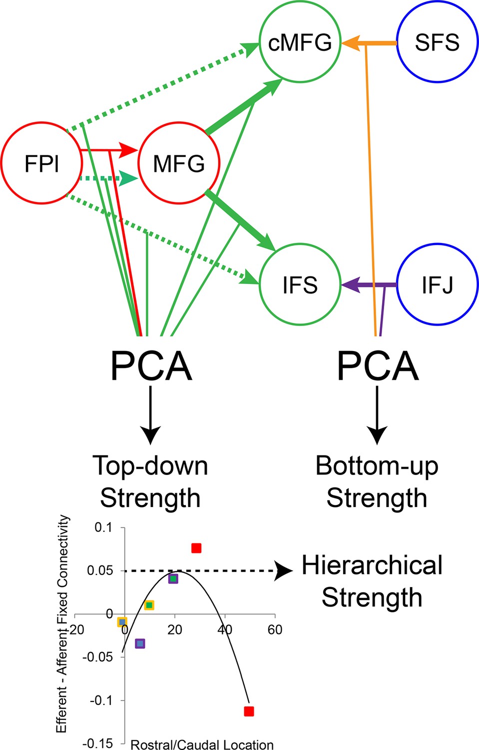
Dynamic causal modeling derived individual difference measures.
Top-down modulations resulting from Temporal Control (red) and Contextual Control (green) were combined using principle components analysis (PCA) to represent top-down strength. Bottom-up modulations resulting from Stimulus Domain (spatial – orange; verbal – purple) were similarly combined using PCA to represent bottom-up strength. The height of the vertex of a parabolic fit of efferent – afferent fixed connectivity by rostral/caudal location was used as a metric of the hierarchical strength of mid LPFC.
Figure 8—figure supplement 3
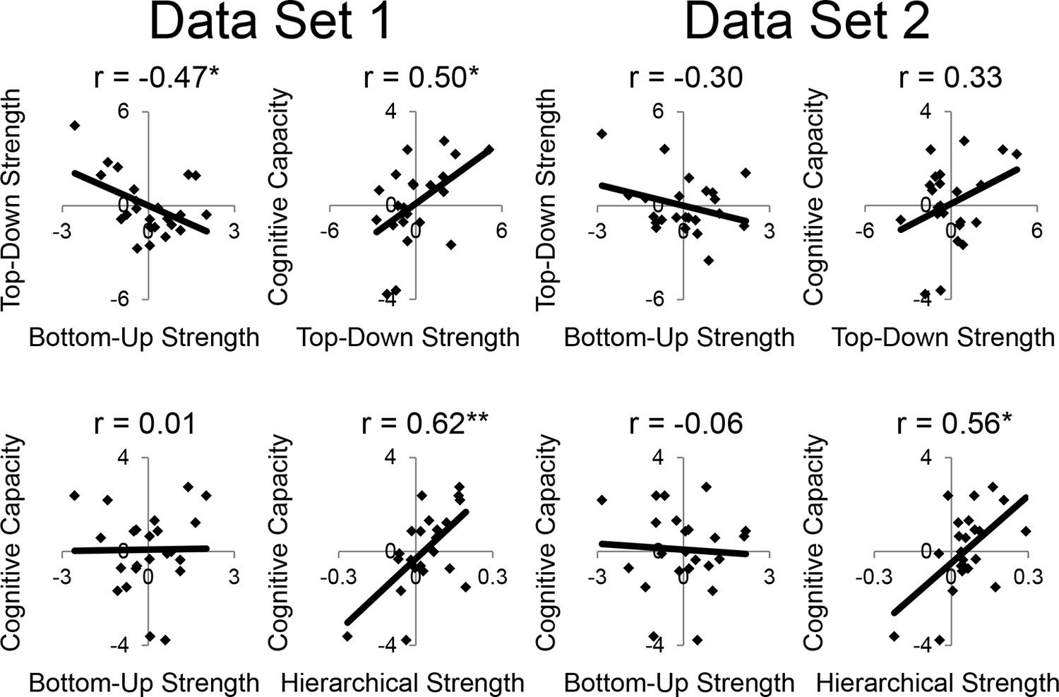
LPFC dynamics and higher-level cognitive ability robustness.
Data were split into two data sets through an alternating runs procedure. Details are otherwise identical to Figure 8 in the main text.
Download links
A two-part list of links to download the article, or parts of the article, in various formats.
Downloads (link to download the article as PDF)
Open citations (links to open the citations from this article in various online reference manager services)
Cite this article (links to download the citations from this article in formats compatible with various reference manager tools)
The hierarchical organization of the lateral prefrontal cortex
eLife 5:e12112.
https://doi.org/10.7554/eLife.12112


