Neural coding in barrel cortex during whisker-guided locomotion
- Janelia Research Campus, Howard Hughes Medical Institute, United States
- IBM Thomas J. Watson Research Center, United States
Figures
Figure 1
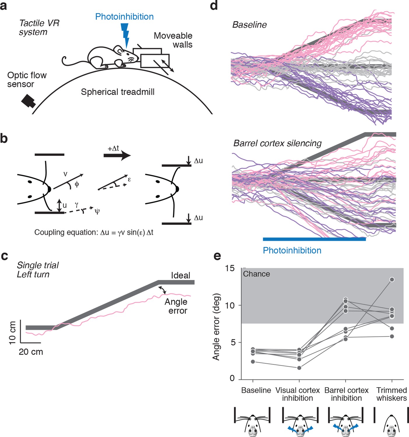
Photoinhibition of barrel cortex during wall tracking.
(a) Side view of a mouse in the tactile virtual reality system. (b) Schematic illustrating closed-loop control of the walls. If the mouse runs at speed v in the direction ϕ in a corridor with a turn angle ψ then wall position u updates according to the coupling equation Δu = γ v sin(ε) Δt where ε = ϕ − ψ the difference, or error, between the run angle and the turn angle, is the gain, and Δt is the time interval. (c) One-left-turn trial. The mouse trajectory (pink) is overlaid on the ideal trajectory (gray), which corresponds to staying in the center of the corridor. The angle error is the difference between the actual and ideal trajectories at the end of the turn. (d) Top, twenty randomly selected running trajectories corresponding to three different turn angles recorded in one session. Bottom, same as above during barrel cortex photoinhibition achieved by photostimulating GABAergic neurons expressing ChR2 (left, pink; straight, gray; right, purple). (e) Average angle error during interleaved trials with no photoinhibition, visual cortex photoinhibition, barrel cortex photoinhibition, and trials with no whiskers. Barrel cortex photoinhibition impaired tracking performance (p = 6.4*10–4 t-test; 8 mice).
Figure 2 with 1 supplement
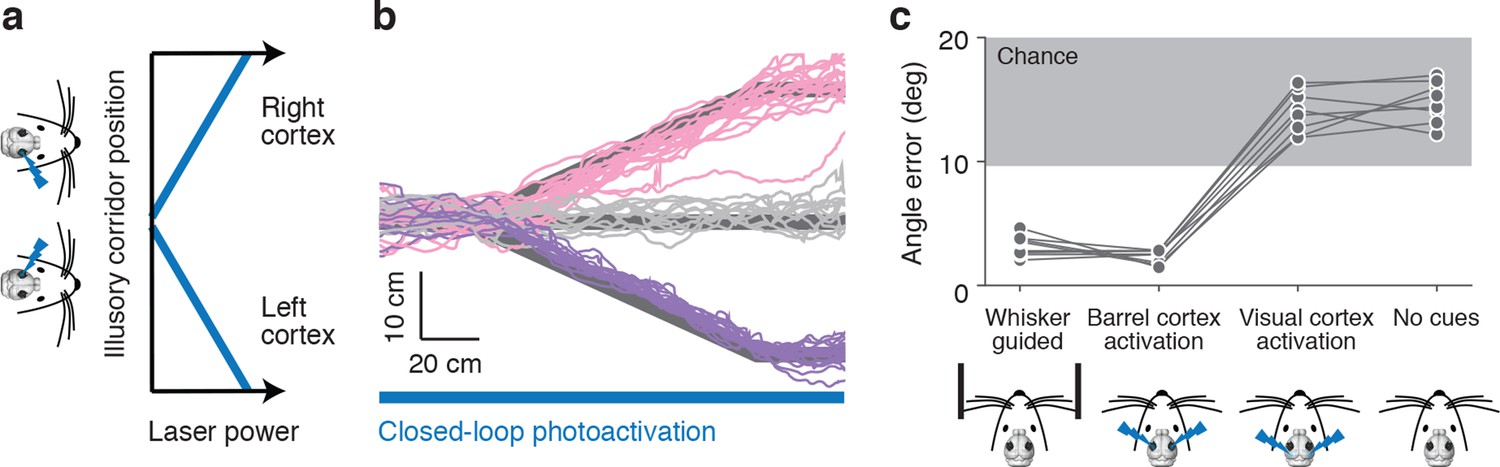
Photoactivation of layer 4 to guide locomotion.
(a) Schematic of an illusory corridor generated with position-dependent photoactivation. In the center of the corridor the laser intensity was zero. On the right side of the corridor the left barrel cortex was stimulated and vice versa. The laser power increased with proximity to the edge of the corridor. (b) Twenty randomly selected running trajectories from three different turn angles during closed-loop photoactivation (left, pink; straight, gray; right, purple). (c) Average angle error during trials of whisker-based wall-tracking, barrel cortex activation, visual or parietal cortex activation, and no cues. Barrel cortex photoactivation was able to drive a behavior resembling wall tracking (p = 1.7*10−8 t-test; 8 mice). Trials with barrel cortex activation, visual or parietal cortex activation, and no whisker or photostimulation cues were randomly interleaved. Trials with whisker-based wall-tracking were recorded in separate sessions. Half of the mice performed the photoactivation sessions after the wall-tracking sessions and half of the mice performed them before.
Figure 2—figure supplement 1
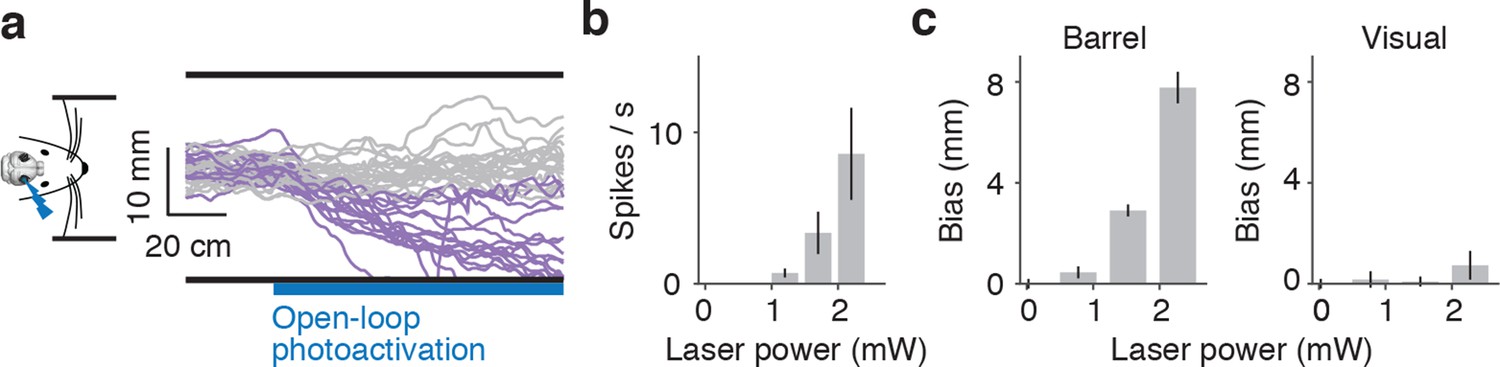
Unilateral activation in mice running in a real corridor.
(a) Twenty randomly selected running trajectories in a straight corridor either with no photoactivation (gray) or with photoactivation of layer 4 of the right barrel cortex (purple). (b) Average activity (6 cells) evoked by photoactivation during cell attached recordings in awake, non-behaving mice as a function of laser power (mean ± SE). (c) Wall distance bias evoked by photoactivation of barrel (left) and visual / pariental cortex (right) as a function of laser power (8 mice, mean ± SE).
Figure 3
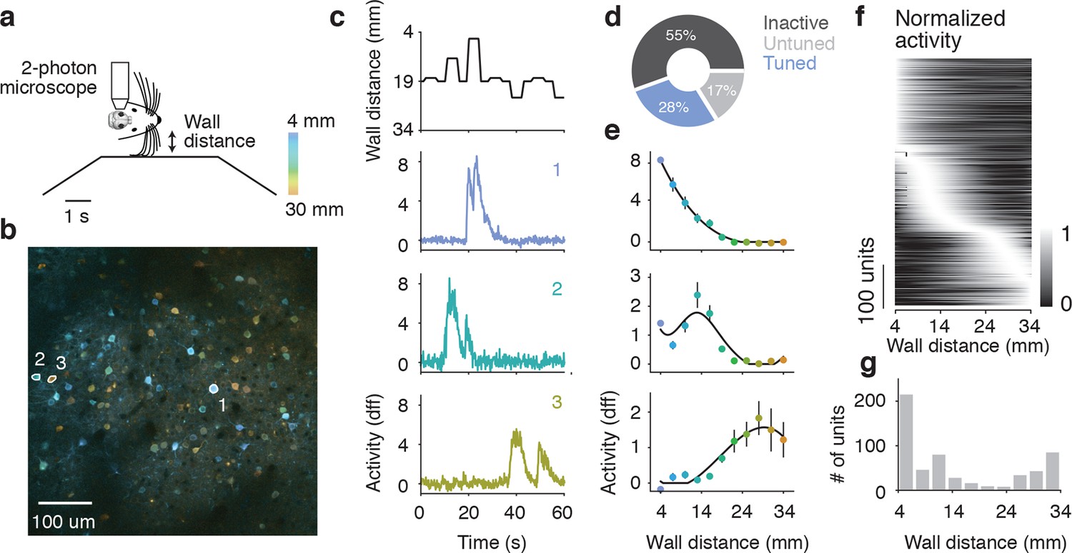
Imaging activity of layer 2/3 neurons during whisker-guided locomotion.
(a) Schematic of two-photon calcium imaging. (b) Overlay of a pixelwise regression map and mean intensity image. Each pixel in the regression map is colored according to its tuning to wall distance; brightness was adjusted according to the r2 value of the tuning. Three example ROIs are highlighted (corresponding to panel c). This imaging region is approximately centered on the C2 barrel (diameter, 300 μm) and contains parts of the neighboring D1 and C1 barrels. (c) Distance from the snout to the wall as a function of time (top) and ΔF/F for three example ROIs (same ROIs as in b). (d) Fraction of neurons in L2/3 that are inactive, tuned, and untuned to the wall distance. (e) Tuning curves to wall distance for example ROIs (mean ± SE over trials). (f) Heatmap of tuning curves normalized by maximum activity across all mice. (g) Histogram of the location of tuning curve peaks.
Figure 4 with 5 supplements

Extracellular electrophysiology during whisker-guided locomotion.
(a) Schematic showing silicon probe recordings during open loop trials. The wall was moved in and out of different fixed distances from the mouse during a period of 4 s. (b) Coronal section through the brain of an Scnn1a-Tg3-Cre x RCL-ChR2-EYFP mouse acquired with green filter showing the barrels. Image acquired with orange filter is superimposed on top showing the track of the silicon probe coated in DiI. Electrolytic lesion is seen at the end of the DiI trace. Location of the probe is identified as C3 barrel. (c) Example spike rasters of regular spiking units during open-loop trials. Each row of the raster corresponds to one trial and each dot corresponds to one spike. The color of each dot represents the position of the wall at the time of the spike. Recordings are performed around C1 and C2 barrels. Only trials with running speed over 3 cm/s are represented. (d) Corresponding tuning curves to wall distance for the spike rasters shown in B (mean ± SE over trials). (e) Histogram of the location of tuning curve peaks. (f) Scatter plot of tuning curve suppression vs. activation. Activation is the difference between peak rate and baseline rate when the wall is out of reach. Suppression is the difference between minimum rate and baseline rate. (g) Heatmaps of z-scored tuning curves for units activated by more than 1 Hz (top) and units suppressed by more than 1 Hz (bottom) sorted by the location of the maximum and minimum wall distances respectively. Units that were both activated and suppressed appear in both plots. (h) Histogram of the tuning modulation, defined as the ratio of the difference between the activation and suppression divided by the sum of the activation and suppression. Units that are just activated have modulation 1, units that are just suppressed have modulation −1, and units that are both activated and suppressed have a modulation near 0. (i) Modulation index as a function of laminar position. Light gray, units classified as layer 2/3; medium gray, layer 4; dark gray, layer 5.
Figure 4—figure supplement 1
Electrophysiological methods.
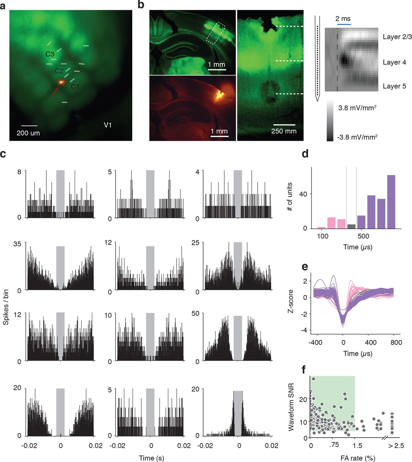
(a) Image acquired with green filter of a whole brain removed from the skull of a Scnn1a-Tg3-Cre x RCL-ChR2-EYFP mouse. Overlay of 13 recordings sites identified by DiI tracing of silicon probe tracks. An image acquired with orange filter and superimposed on top for one example. The recording site is shown by arrow. (b) Illustration of three complementary methods used for identification of the depth of recorded units. Left: Coronal section of barrel cortex acquired with green and orange filters showing with dotted square the location of recording site. Center: Blown-up portion of the same area of the coronal section (turned rotated by 39 degrees) taken with green filter showing of L4 barrels. The location of two electrolytic lesions on top and bottom electrodes and the center of layer 4 are marked with dashed white lines. Right: Current source density trace used to identify the middle of Layer 4 as a short-time (<3 ms) minimum. The schematics of electrodes positions on the silicon probe that is aligned with the centers of the top and bottom lesions. (c) Inter-spike-interval distributions for units presented in Figure 4 and Figure 5. (d) Histogram of spike widths. Fast spikers (< 350 μs): pink, intermediate: gray, and regular spikers (> 450 μs): purple). (e) Z-scored waveforms from all units. (fast spikers: pink, intermediate: gray, regular spikers: purple). (f) Scatter plot of waveform SNR against ISI false alarm rate. The area shown by colored square corresponds to accepted units with SNR > 6 and false alarm rate < 1.5%
Figure 4—figure supplement 2
Lamina distribution of units.
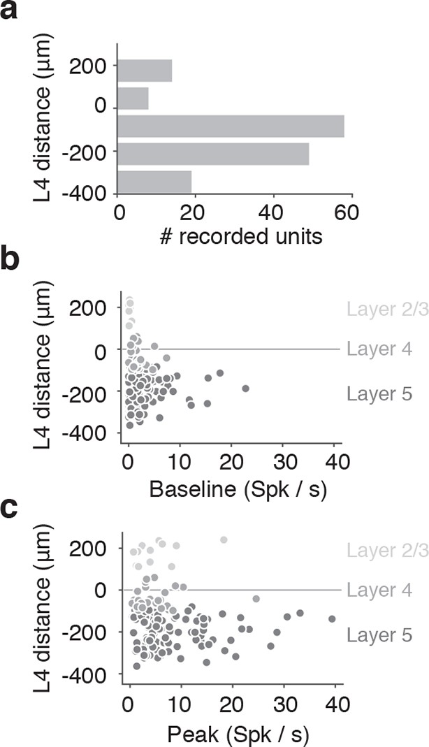
(a) Distribution of the location of regular spiking units by depth relative to the middle of Layer 4. (b) Depth distribution of a baseline spike rate of regular spiking units during locomotion (speed over 3 cm/s). Light gray, units classified as layer 2/3; medium gray, layer 4; dark gray, layer 5. (c) Depth distribution of a peak spike rate of regular spiking units during locomotion (speed over 3cm/s). Light gray, units classified as layer 2/3; medium gray, layer 4; dark gray, layer 5.
Figure 4—figure supplement 3
Comparison of open-loop and closed-loop tuning curves.
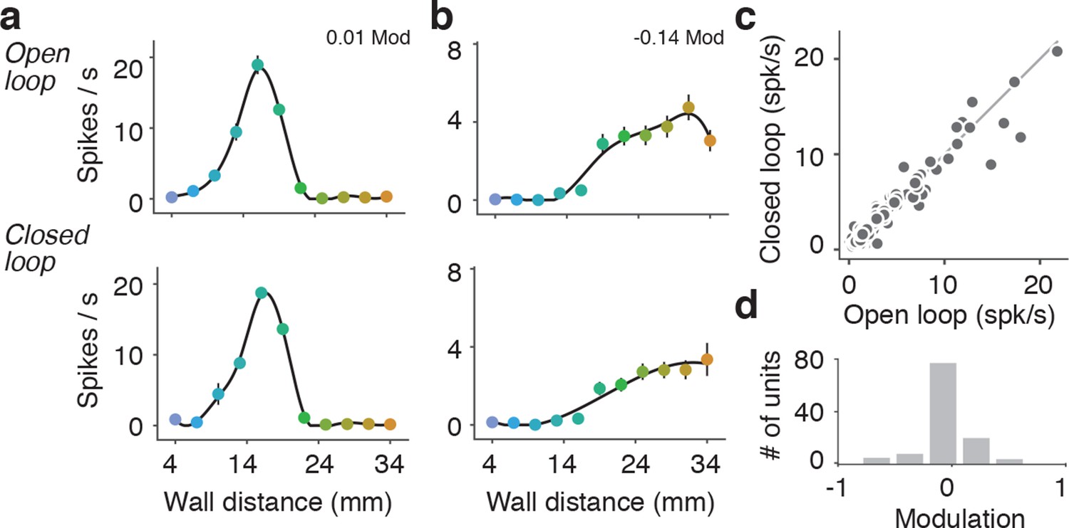
(a) Open-loop and closed-loop tuning curves for a regular spiking unit that gets activated by the wall. (b) Open-loop and closed-loop tuning curves for a unit that gets suppressed by the wall. (c) Scatter of the mean spiking rate of open-loop and closed-loop tuning curves. (d) Histogram of open vs. closed-loop modulation index which is the difference in open-loop and closed-loop spiking rates divided by the sum of open-loop and closed-loop spiking rates. Units that respond more during open loop trials have positive modulation, units that respond more during closed loop trials have negative modulation, and units that responded equally to both open and closed loop trials have a modulation of 0.
Figure 4—figure supplement 4
Effects of running speed on activity and wall distance tuning.
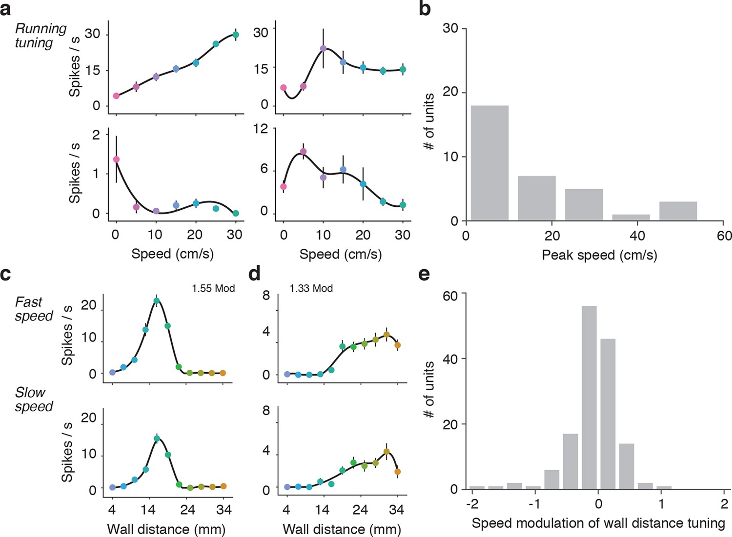
(a) Four example units that showed significant tuning to running speed when the wall was out of reach. The activity of the top left unit increased linearly with speed over a large range, the activity of top right unit increased rapidly and then saturated at low speeds, the activity of the bottom right unit peaked at low speeds and then decreased at higher speeds, and the activity of bottom left unit decreased with running speed. (b) Histogram of the peak speed tuning for units significantly tuned to speed (31%; 46/148) from the population used in Figure 4. (c) Example wall distance tuning curve while the mouse is running in fast trials (top) and slow trials (bottom). Fast and slow trials were split based on the median of the trial speeds in trials when the mouse was running. This unit is the same as used in Figure 4—figure supplement 3a). (d) Example wall distance tuning curve while the mouse is running fast trials (top) and slow trials (bottom). This unit is the same as used in Figure 4—figure supplement 3b). (e) Histogram of the modulation of wall distance tuning by speed for all 148 units. This index was the log of the gain parameter that describes a multiplicative scaling of the slow tuning curve to the fast tuning curve. Units that are more active during fast running have positive modulation indices, units that are less active during fast running have negative indices.
Figure 4—figure supplement 5

Tuning to ipsilateral and contralateral wall distance.
(a) Example spike raster of regular spiking unit in open-loop trials when the wall is contralateral (top) or ipsilateral to the recording site (bottom). Only epochs with running speed over 3 m/s are represented. This neuron was activated by interactions with the wall. (b) Corresponding tuning curves recorded during locomotion (running speed over 3 m/s). (c,d) Same as a, b for a suppressed regular spiking unit. (e) Scatter plot of range of spiking of ipsilateral vs. contralateral tuning curves. The range of spiking is the difference between the maximum and minimum of the tuning curve. (f) Histogram of laterality modulation index, which is the difference in contralateral range and ipsilateral range divided by the sum of the contralateral range and ipsilateral range. Units that respond only to the contralateral wall have modulation 1, units that respond only to the ipsilateral wall have modulation −1, and units that respond to both the contralateral and ipsilateral wall have a modulation near 0.
Figure 5

Tuning to direction of wall movement.
(a) Example spike rasters of regular spiking units that showed strong modulation by wall direction during open-loop trials during locomotion (running speed over 3 cm/s). (b) Spike rate as a function of time during epochs when wall is moving towards/away from the mice for the same regular spiking units as in a. (c) Heatmap of time profiles curves normalized by maximum for symmetric and asymmetric units, sorted by time to peak. (d) Scatter of the range of spike rates as the wall moved towards and away from the mouse. The range of spike rates is the difference between the maximum and minimum rate during the 1 s when the wall was moving towards or away from the mouse. (e) Histogram of direction modulation index, which is the range difference in spike rates during wall movement towards and away from the mouse divided by the sum of the towards range and away range. Units that respond only when the wall approaches have modulation 1, units that respond only when the wall moves away have modulation −1, and units that respond to both the wall approaching and moving away have a modulation near 0.
Download links
A two-part list of links to download the article, or parts of the article, in various formats.
Downloads (link to download the article as PDF)
Open citations (links to open the citations from this article in various online reference manager services)
Cite this article (links to download the citations from this article in formats compatible with various reference manager tools)
Neural coding in barrel cortex during whisker-guided locomotion
eLife 4:e12559.
https://doi.org/10.7554/eLife.12559


