Multiplexed coding by cerebellar Purkinje neurons
- Okinawa Institute of Science and Technology, Japan
- Erasmus Medical Center, The Netherlands
- Hertie Institute for Clinical Brain Research, University of Tübingen, Germany
Figures
Figure 1 with 1 supplement
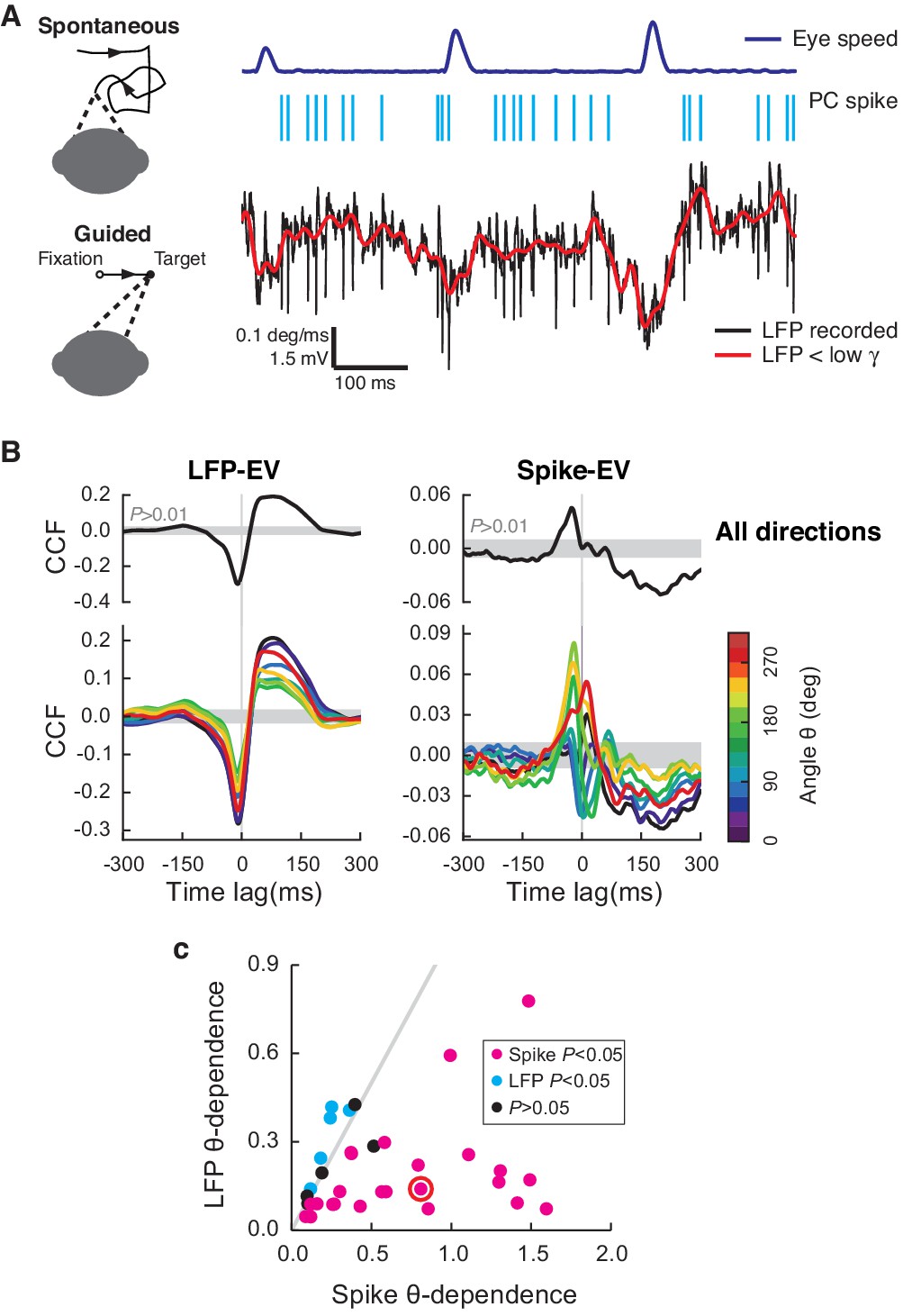
Cerebellar LFP and PC spikes correlate differently with saccadic eye movements.
(A) Left: Schematics of eye motion tasks. Right: Simultaneously recorded eye speed, PC spike train, and LFP. Both the recorded (black) and filtered LFP below the low-γ frequency (red) are shown, but only the latter was analyzed. (B) CCFLFP-EV and CCFSpike-EV computed with EV (Top) and eye speed in the direction with the angle θ (Bottom). Shaded regions represent the 99% confidence interval. Data are normalized as described in the Materials and methods and plotted as mean ± SEM. (C) θ-dependent variability of CCFLFP-EV (x-axis) versus CCFSpike-EV (y-axis). CCFSpike-EV varied significantly more (p<0.05, t-test) than CCFLFP-EV in 74% (n = 25; magenta), and less in 15% (n = 5; cyan) of all recordings. No difference was found in the rest (n = 4; black). Error bars are omitted for clarity. The gray line represents equal variability. The red circle denotes data in A and B.
Figure 1—figure supplement 1
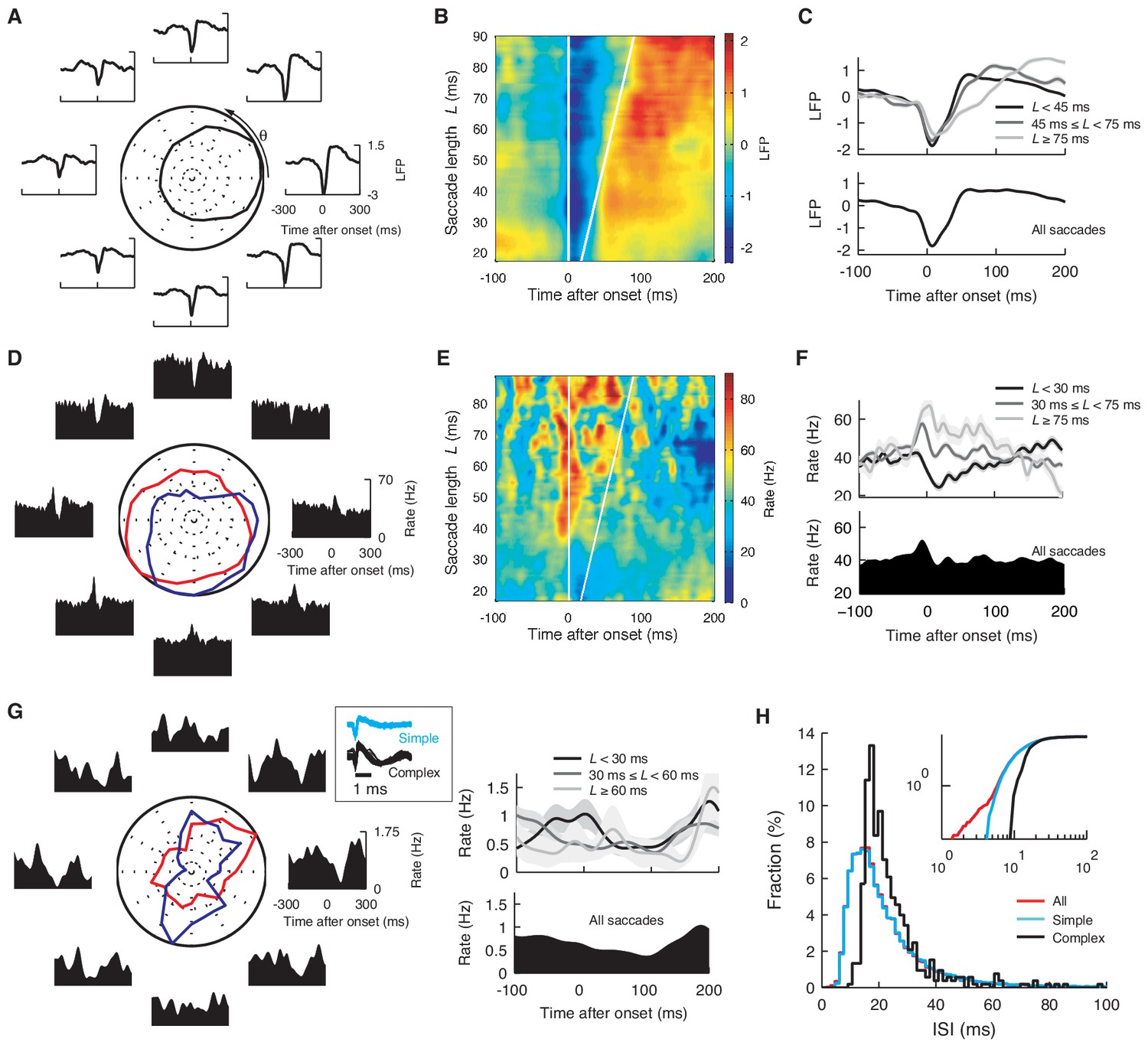
Saccade angle and duration dependence of the onset-triggered average LFP, simple and complex spikes.
(A) Onset-triggered average LFP with different saccade angle θ and, (B) L. Each data point at θ or L represents the average over [θ − 45º, θ + 45º] or [L − 4 ms, L + 4 ms]. The LFP was normalized by its standard deviation. In (A) the curve in the center represents the normalized peak-to-peak amplitude of the average LFP. In (B) white lines mark the saccade beginning and end, respectively. (C) The average LFP for the different saccade lengths (top), and for all the saccades (bottom). (D, E, F) The same plots as (A–C) for the firing rate. In (D) red and blue lines represent normalized maximal and minimal firing rates, respectively. The rate was computed with a Gaussian smoothing kernel of σ = 10 ms. Note that waveforms in (A) and (D) are similar to CCFs in Figure 1B. (G) Firing rate of complex spikes, computed with σ = 25 ms, varying with θ (left) and L (right). The boxed insert shows spike waveforms. (H) Histograms of ISIs after simple (cyan), complex (black), and all spikes (red). Note that the simple and all-spike cases are nearly identical while the complex spike case is shifted, reflecting pauses after complex spikes. Cumulative distributions (inset) show that the all-spike case has a small number of short ISIs < 5 ms, caused by complex spikes that immediately follow simple spikes. Data are mean ± SEM. The data are the same as in Figure 1A,B.
Figure 2 with 1 supplement
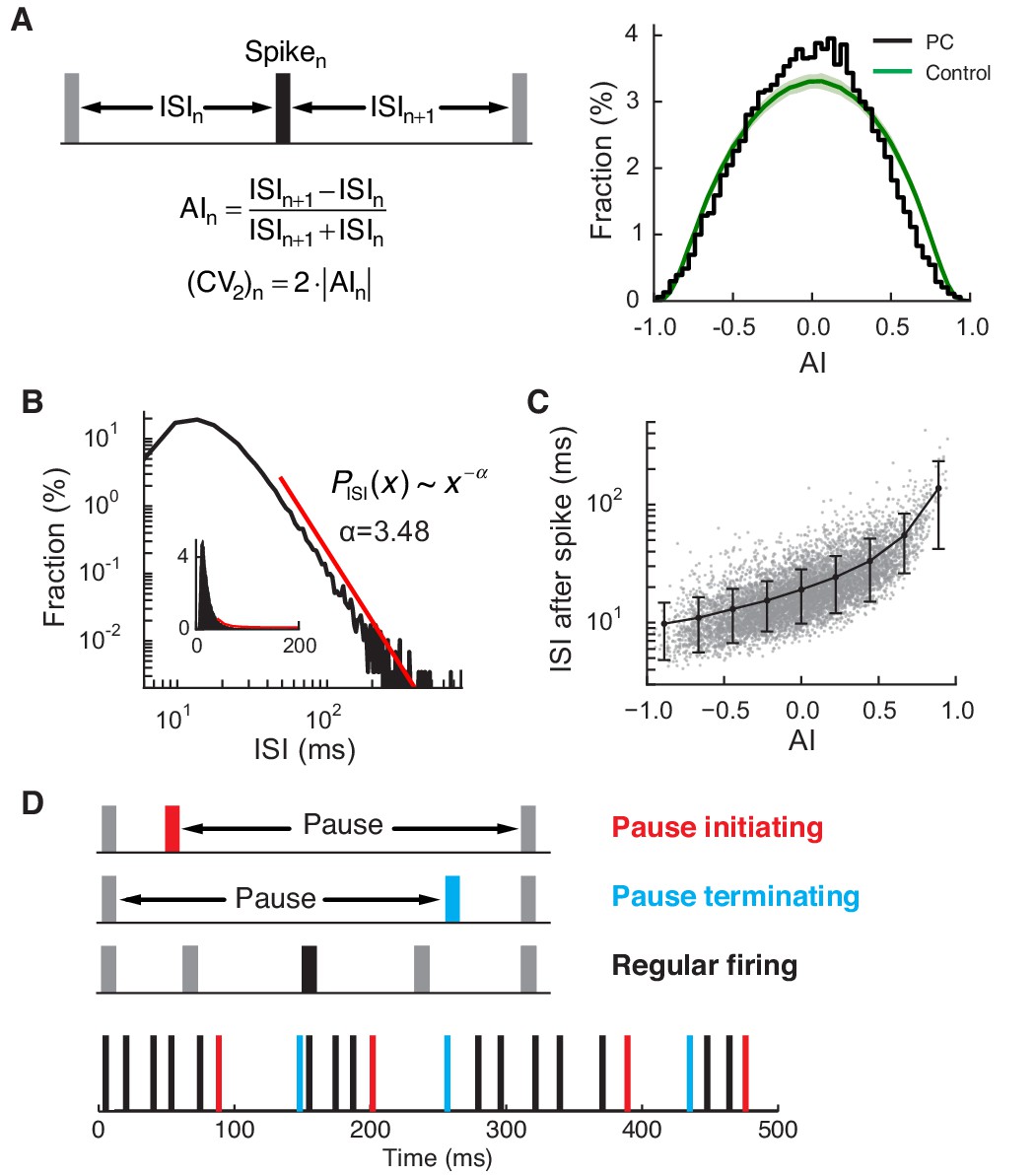
Regular and pause spikes in the PC spike train.
(A) Left: The ISI asymmetry index (AI) measures local variability at each spike and is related to the local coefficient of variation (CV2). Right: Distribution of AI for PC spikes (black) and rate-matching control spike train (green, mean ± SD). Significantly more PC spikes occurred around AI ≈ 0. (B) The ISI histogram with a fitted power-law tail (red). Inset: the same histogram and tail in linear scales. (C) ISI after each spike vs. AI. The black line represents mean ± SD in each bin (center = [-0.8, -0.6, …, 0.8], width = 0.2). (D) Top: Three types of spiking pattern classified by their AI and associated ISI length. Bottom: Examples of pause and regular spikes in an actual PC spike train. Data are the same as in Figure 1A,B.
Figure 2—figure supplement 1
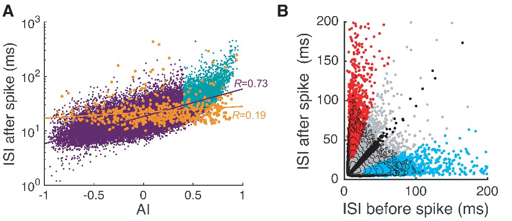
Complex and simple spike pauses.
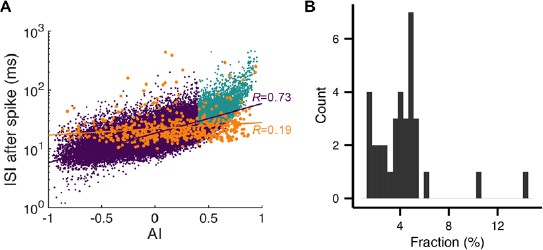
(A) ISI after each spike vs. AI for all spikes. Orange dots are complex spikes. Light blue dots are pause-initiating spikes selected based on the AI value and ISI size (see next section and Materials and methods for details). Lines represent correlation coefficients R. Here the fraction of selected pauses caused by complex spikes is 1.75%. (B) ISIs after spikes vs. ISIs before spikes. Red, cyan, and black dots are pause-initiating, -terminating, and regular spikes, respectively. The rest of the spikes are gray dots. Contours represent log10 (density). Note that the density becomes stretched along x- and y-axes and develops two tails as the ISI becomes larger. Data are the same as in Figure 2.
Figure 3 with 4 supplements

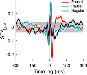
Pause and regular spikes correlate differently with the LFP.
(A) Left: STALFP of the pause-initiating (red), -terminating (cyan), and regular spikes (black). The grey region is the 99% confidence interval. h is the peak-to-peak amplitude and shown for pause-terminating spikes. Right: STALFP of randomly selected spikes (black) and all spikes (green). Data are mean ± SEM. (B) Relative STA amplitude, h, to that of all spikes (hAll) for each spike category. (C) Phase distribution of the β/γ LFP at the pause, regular, and randomly selected spikes (thick: histogram, thin: kernel-estimated density). φ denotes location of the peak, shown for the pause-initiating spike. (D) Pair phase consistency (PPC) for each spike category. (E) Peak phases for the pause-initiating (x-axis) and pause-terminating spikes (y-axis) in all data. Grey and red lines represent φPauseT = φPauseI and φPauseT = φPauseI + 278.3º, respectively. In (C) and (E), **p<10–5 (Wilcoxon rank-sum test). Data in (A), (D), and (E) are the same as in Figure 1A,B.
Figure 3—figure supplement 1

STALFP with different selection criteria for pause spikes.
We used a similar scheme to choose pause and regular spikes as in Figure 3, but varied the AI and CV2 thresholds to change the number of spikes in each group from 7.5% to 37.5% of all spikes in increments of 7.5%. (A) STALFP of the pause-initiating, -terminating, and regular spikes. Note that the fast fluctuating part of the STALFP remains robust in the case of pause spikes. Data are the same as in Figure 3A. (B) Amplitude of the STALFP of the β/γ band LFP vs. the number of spikes in each group, for all cells. Amplitudes are all normalized by those of STALFP from all spikes (dotted line). Data are mean ± SD.
Figure 3—figure supplement 2
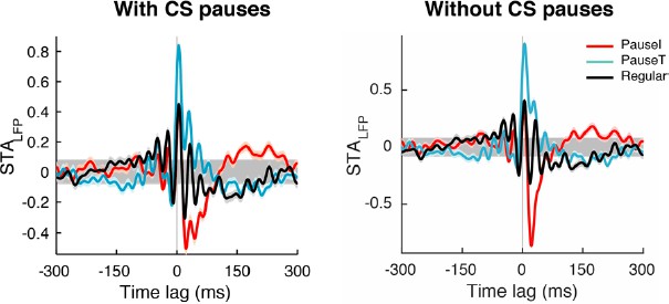
STALFP in other data sets.
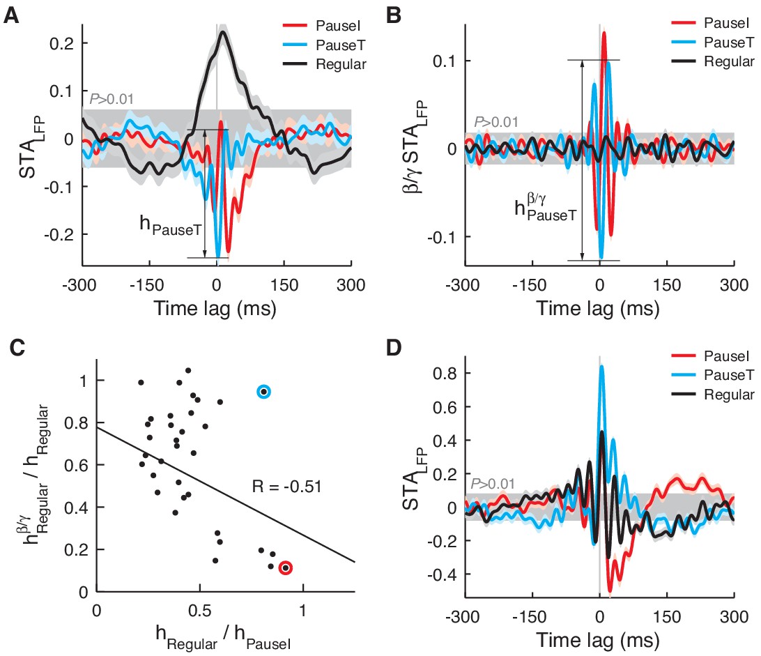
In a minority of cases (n = 7), STALFP of the regular spikes (AI ≈ 0) had a comparable (>60%) amplitude to that of pause spikes (A). However, the amplitude significantly diminished when STALFP was recomputed with the LFP in the β/γ band (B). The amplitude of the regular spike STALFP in the β/γ band (hβ/γRegular) was negatively correlated with the original amplitude (hRegular) (C) suggesting that, when regular spikes are significantly coupled to the LFP, they prefer time scales slower than the β frequency. In C, the red circle corresponds to data in A and B while the cyan circle is a single, exceptional case where hRegular remained relatively large (D). For pause spikes, the original amplitude is mostly retained as hβ/γ/horig = 0.86 ± 0.13 (mean ± SD).
Figure 3—figure supplement 3
Spike-LFP phase locking in other frequency bands.
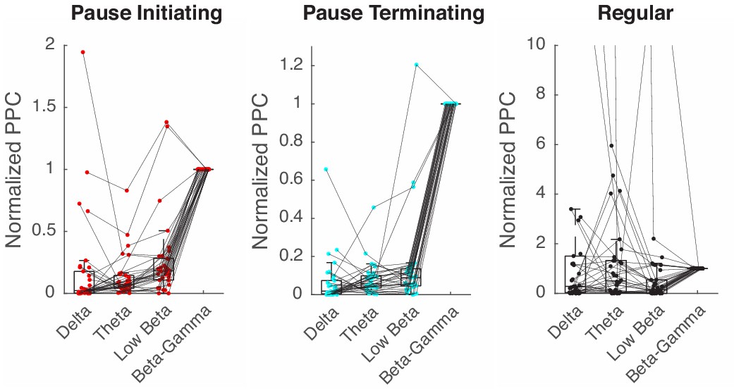
PPC is computed with the band-passed LFP in the β/γ (15–42 Hz), low β (10–15 Hz), θ (4–10 Hz), and δ (<4) band, and all normalized by values in the β/γ case.
Figure 3—figure supplement 4
STALFP depends on LFP spectral properties.
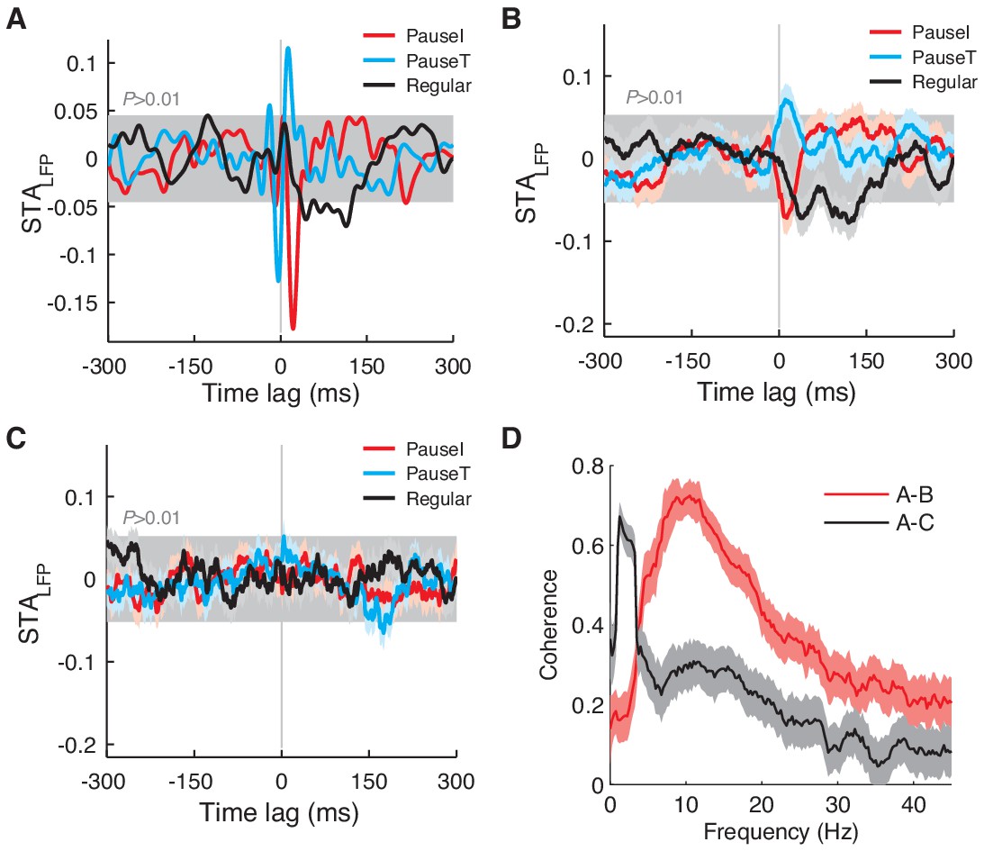
(A–C) STALFP based on the LFP from the same electrode as the spike signal (A) and on the LFP from two other electrodes. (B,C) In B, STALFP for pause and regular spikes has distinct waveforms similar to A, but not C. Coherence between LFPs in (A) and (B) is significantly higher than between (A) and (C). Note that we omitted the final stage of LFP filtering (< 42Hz) in (B) and (C), nonetheless, the spike waveform is negligible. (D) Coherence between LFPs from different locations. The LFP shown in B is significantly more coherent with the LFP in (A) than the LFP in (C) in the higher frequency range (>4 Hz), which underlies the difference in STALFP shown in (A–C). Electrodes for (B) and (C) were both 1 mm distant from the spike electrode in A. The difference between (B) and (C) suggests that the relevant signal also depends highly on the vertical electrode position. Coherences and their confidence intervals (99%, light color) were computed with the chronux toolbox (http://chronux.org).
Figure 4 with 1 supplement

Pause spikes and β/γ LFP encode motion timing.
(A) Eye speed (Top) and β/γ LFP (Bottom) aligned with saccade onset. Black lines represent an average over all saccades (grey, n = 865). (B) Phases of the β/γ LFP at saccade onset for the same data. (C) Top: Spike trains for pause-initiating, -terminating, and regular spikes aligned with onsets of randomly subselected saccades (n = 289). Light colored regions represent periods with significantly reliable firing (jp(t)<0.05, see Materials and methods). Bottom: Z-score for spike occurrence, smoothed by a gaussian kernel (σ = 5 ms). (D) Spike reliability of pause and regular spikes in all data. *p = 0.0229, 0.0193 (Wilcoxon rank-sum test). (E) LFP phase reliability versus spike reliability. The two were significantly correlated (red and black line) for pause-initiating and regular spikes (p = 9.3074 × 10⁻⁶, 0.0012; Fisher’s z-test), but not for pause-terminating spikes (p = 0.0912), due to some recordings with low spike reliability but high LFP reliability. Data in (A–C) are the same as in Figure 1A,B.
Figure 4—figure supplement 1
Peak firing of pause and regular spikes during saccades.
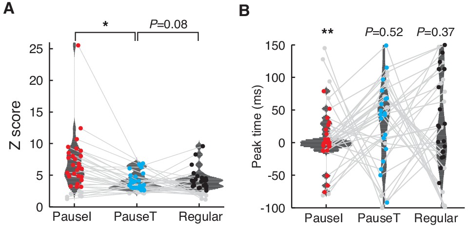
(A) Distribution of the peak Z-score for the firing probability of the pause versus regular spikes. We used a time window from −100 ms to 150 ms around saccade onset and the baseline was estimated with 200 randomized controls. Only significant peaks (colored dots) were used to compute the distributions (p<0.01, t-test; n = 27, 19, and 19 for pause-initiating, -terminating, and regular spikes, respectively). Gray dots represent insignificant data sets. *p = 0.0061 (Wilcoxon rank-sum test) (B) Distribution of Z-score peak timing. The mean timing ± SD for pause-initiating, -terminating, and regular spikes are 1.48 ± 24.5 ms, 15.6 ± 43.0 ms, and 13.9 ± 70.6 ms. Colored and gray dots represent significant and insignificant peaks, respectively. Only the distribution of pause-initiating spikes is significantly different from a uniform distribution (**p = 6.7353 × 10⁻⁴, Kolmogorov-Smirnov test).
Figure 5 with 1 supplement
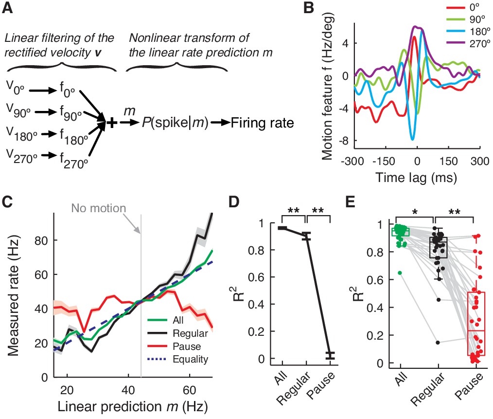
PC firing rate linearly encodes motion kinematics.
(A) Schematics of the eye motion-to-rate inverse model. (B) Example motion feature. (C) Predicted vs. measured firing rate for all (green), regular (black), and pause (red) spikes. The rates of pause and regular spikes are rescaled to match those of all spikes to compensate for subsampling. The dotted line represents equality. (D) Goodness of fit R2 for the linear prediction to actual rate. **p<10-30 (Wilcoxon rank-sum test). (E) R2 for all cells. Error bars are omitted and box plots are for means. *p<10-6, **p<10-11 (Wilcoxon rank-sum test). Error bars represent SEM. Data in B–D are the same as in Figure 1A,B.
Figure 5—figure supplement 1
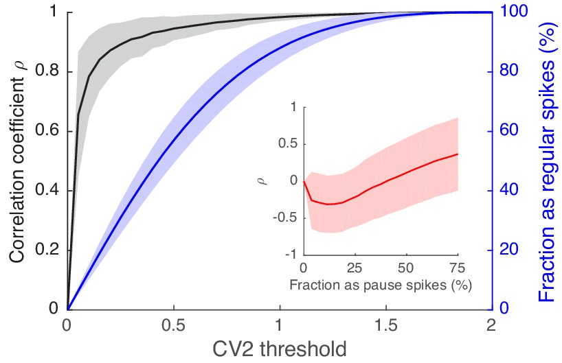
Spikes with high regularity have a spike-eye motion correlation that is very similar to that of the full spike train.
Black traces are correlation coefficients of the CCFSpike-EV, computed in eight eye movement directions, between the full spike train and regular spikes selected based on the CV2 threshold (x-axis). The blue line is the fraction of regular spikes out of all spikes. The inset contains the same correlation coefficients for pause spikes vs. the fraction of pause spikes out of all spikes. Varying numbers of pause spikes were selected by varying the AI threshold as in Figure 3—figure supplement 1. Data are mean ± SD.
Author response image 1
Author response image 2
Author response image 3
Author response image 4

Author response image 5

Download links
A two-part list of links to download the article, or parts of the article, in various formats.
Downloads (link to download the article as PDF)
Open citations (links to open the citations from this article in various online reference manager services)
Cite this article (links to download the citations from this article in formats compatible with various reference manager tools)
Multiplexed coding by cerebellar Purkinje neurons
eLife 5:e13810.
https://doi.org/10.7554/eLife.13810


