Neural oscillations as a signature of efficient coding in the presence of synaptic delays
- Institute of Science and Technology Austria, Austria
- École Normale Supérieure, France
- National Research University Higher School of Economics, Russia
Figures
Figure 1
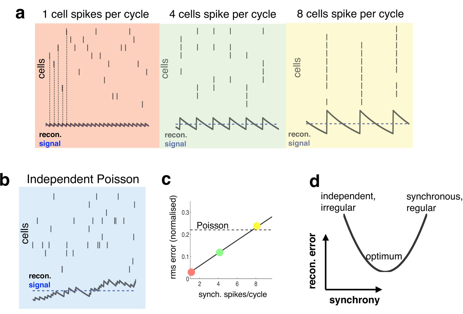
Relationship between synchrony and coding accuracy.
(a) Each panel illustrates the response of 10 neurons. An encoded sensory variable is denoted by a horizontal blue line. Each spike fired by the network increases the sensory reconstruction by a fixed amount, before it decays. Greatest accuracy is achieved when the population fires at regular intervals, but no two neurons fire together (left). Coding accuracy is reduced when multiple neurons fire together (middle and right panels). (b) Same as panel a, but where neurons show independent poisson variability. (c) Reconstruction error (root-mean squared error divided by the mean) for a regular spiking network shown in panel a, versus the number of synchronous spikes on each cycle. A horizontal line denotes the performance when neurons fire with independent Poisson variability. (d) Cartoon illustrating tradeoff between trade-off faced by neural networks.
Figure 2

Efficient coding in a recurrent neural network.
(a) Schematic of network. Inhibitory recurrent connections are represented by an open circle. Excitatory feed-forward connections are represented by closed circles. (b) Stimulus (blue) and neural reconstruction (black) on a single trial. The spikes and membrane potential for each cell are shown in separate rows. Vertical dashed lines illustrate how each spike alters the neural reconstruction. (c) Same as (b), but with a constant input (also note the change of temporal scale). (d–e) Distribution of inter-spike intervals in population (d) and single-cell (e) spike trains.
Figure 3
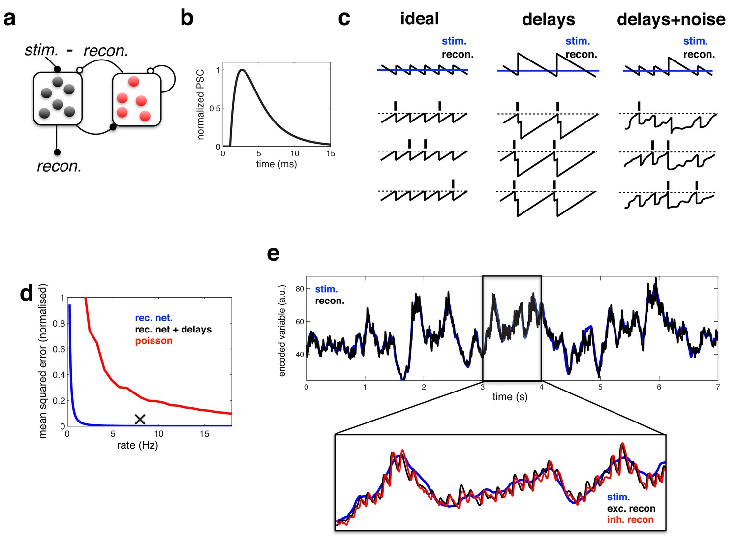
Coding performance of an excitatory/inhibitory network with synaptic delays.
(a) Schematic of network connectivity. Excitatory neurons and inhibitory neurons are shown in black and red, respectively. Connections between different neural populations are schematised by lines terminating with solid (excitatory connections) and open (inhibitory connections) circles. (b) The postsynaptic current (PSC) waveform used in our simulations. (c) Schematic, illustrating how delays affect the decoding performance of the network. (d) Mean-squared reconstruction error (normalized by variance of encoded signal) versus mean firing rate for an ‘ideal’ efficient coding network with instantaneous synapses (blue), an efficient coding network with finite synaptic delays (black cross) independent Poisson units whose firing rate varies as a fixed function of the feed-forward input (red). (f) Stimulus and neural reconstruction for the recurrent network, with synaptic delays. (inset) Excitatory (black) and inhibitory (red) neural reconstructions, during a short segment from this trial.
Figure 4
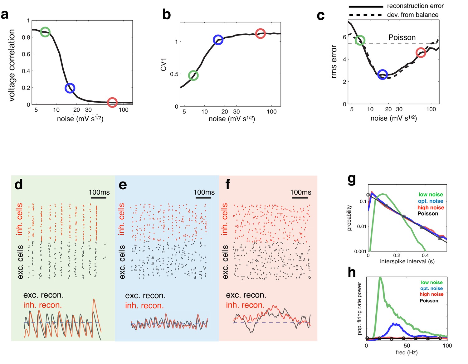
Effect of varying noise amplitude on network dynamics and coding performance.
(a) Pairwise voltage correlations, versus injected noise amplitude. (b) Coefficient of variation in inter-spike intervals, versus injected noise amplitude. (c) Root-mean-square (rms) reconstruction error (solid line), plotted alongside rms difference between excitatory and inhibitory reconstructions (dashed line), versus injected noise amplitude. Horizontal dashed line shows the rms reconstruction error for a population of Poisson units with matched firing rates. (e–f) (upper panels) Spiking response of inhibitory (red) and excitatory (black) neurons with low (d), medium (e), and high (f) noise amplitude (indicated by open circles in panels a–c). (lower panels). Inhibitory (red) and excitatory (black) neural reconstructions, alongside target stimulus (blue dashed line). (g) Distribution of single-cell inter-spike intervals in each noise condition. The prediction for a population of Poisson units is shown in black. Note the log-scale. (h) Power spectrum of population firing rate, in each noise condition. The power spectrum for a population of Poisson units is shown in black.
Figure 5
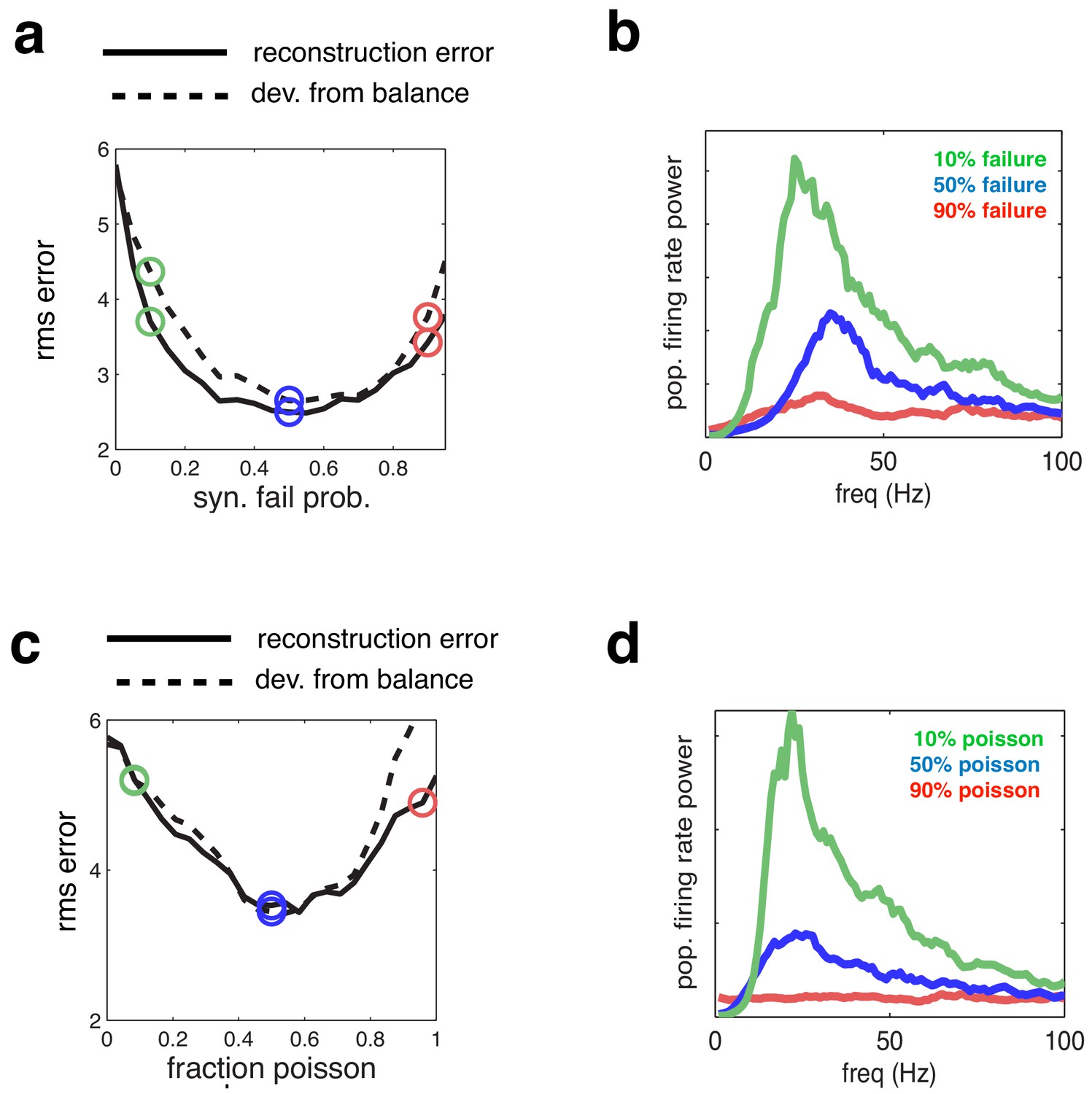
Effect of varying network synchrony in different ways.
(a–b) Effect of varying the probability of synaptic failure. Panel a shows the root-mean-square (rms) reconstruction error (solid line), plotted alongside the rms difference between excitatory and inhibitory reconstructions (dashed line). Panel b shows the firing rate spectrum with varying probability of synaptic failure (indicated by open circles in panel a). (c–d) Same as panels a–b, but where we varied the fraction of cells that fired randomly (i.e. with Poisson spike trains).
Figure 6
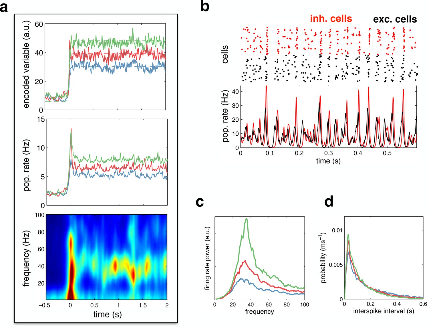
Spiking response to a constant input.
(a) (top) Neural reconstruction (solid lines) of a presented constant stimulus (dashed lines), before and after stimulus onset. Low, medium and high amplitude stimuli are shown in blue, red and green, respectively. (middle) Population firing rate, for each stimulus amplitude. (bottom) Spectrogram of population firing rate. (b) The upper panel shows a raster-gram of excitatory (black) and inhibitory (red) responses, during a 0.6 s period of sustained activity. The lower panel shows the instantaneous firing rates of the excitatory and inhibitory populations. (c) Power spectrum of excitatory population firing rate during the sustained activity period, for each stimulus amplitude. (d) Average distribution of single-cell inter-spike intervals, for each stimulus amplitude.
Figure 7
Voltage responses in response to a constant input.
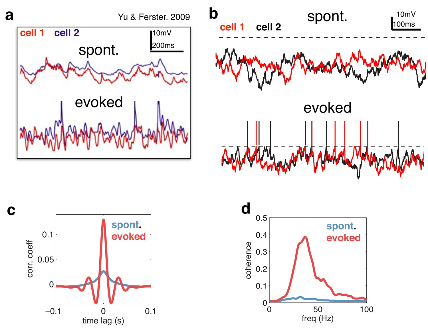
(a) Data from Yu & Ferster (Neuron, 2010), showing voltage traces of two V1 cells, in the absence (top), and presence (bottom) of a visual stimulus. (b) Voltage traces of two cells in the model in absence (top) and presence (bottom) of a feed-forward input. (c) Average pairwise cross-correlation between membrane potentials, in spontaneous and evoked condition. (d) Average coherence spectrum between pairs of voltage traces, in spontaneous and evoked condition.
Figure 8
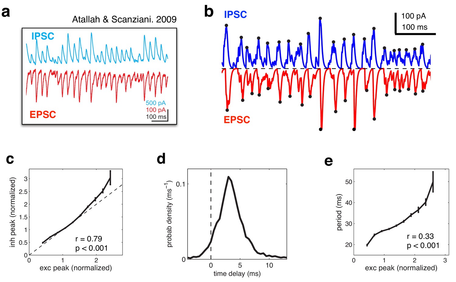
Balanced fluctuations in excitatory and inhibitory currents.
(a) Data from Atallah & Scanziani (Neuron, 2009), showing inhibitory (blue) and excitatory (red) postsynaptic currents. (b) Inhibitory (blue) and excitatory currents (red) in the model, in response to a constant feed-forward input. Black dots indicate detected peaks. (c) Amplitude of inhibitory current versus magnitude of excitatory currents on each cycle. (d) Distribution of time lags between excitatory and inhibitory peaks. (e) Period between excitatory peaks, versus the peak amplitude on the previous oscillation cycle.
Figure 9
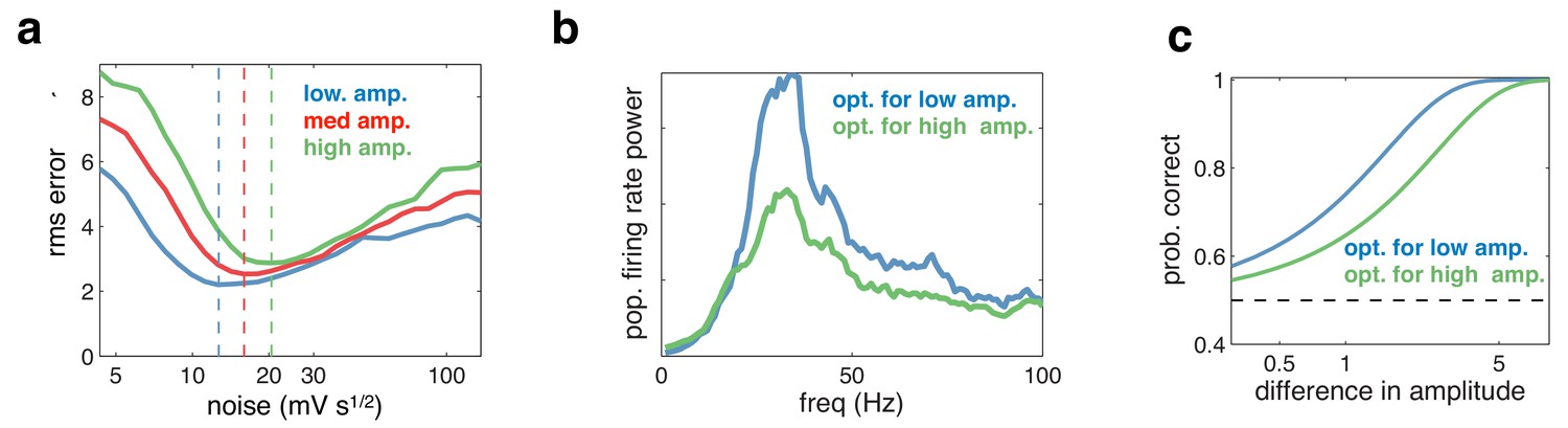
Effect of varying the input amplitude.
(a) Root-mean-square (rms) reconstruction error versus injected noise amplitude with three different input amplitudes. The optimal noise level in each condition is denoted by vertical dashed lines. (b) Power spectrum of population firing rate, in response to a low amplitude input. The blue curve corresponds to when the network is optimised for the low amplitude input, the green curve for when it is optimised for higher amplitude input. (c) Fractional performance in discriminating between two 100 ms input segments, equally spaced around the low amplitude input. Performance is best in the condition with strongest oscillations.
Figure 10
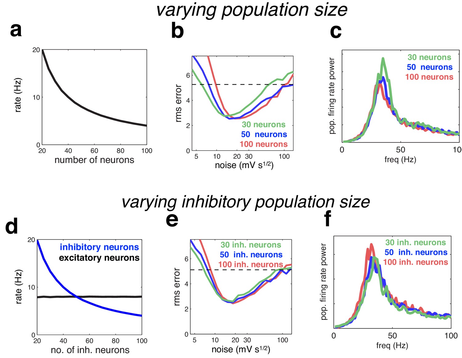
Effect of varying population size.
(a) With recurrent and feed-forward weights held constant, neural firing rates are inversely proportional to population size. (b) Root-mean-squared (rms) reconstruction error versus added membrane noise, for three population sizes. A horizontal line denotes the performance of a Poisson spiking network with matching population firing rate. (c) Power spectrum of population of population firing rate, for each network size (in each case, the noise was set to its optimal value). (d–e) Same as panels a–c, but where we only varied the size of the inhibitory population.
Figure 11
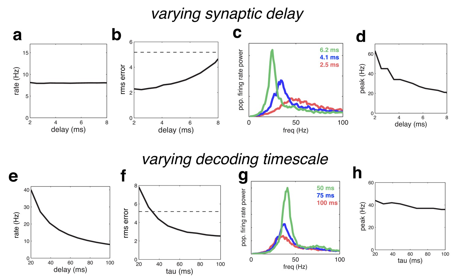
Effect of varying the network time constants.
(a) Neural firing rates versus the synaptic delay. (b) Root-mean-squared (rms) reconstruction error versus the synaptic delay. A horizontal line denotes the performance of a Poisson spiking network with matching population firing rate. (c) Power spectrum of population firing rate, for three different settings of the synaptic delay. (d) Peak oscillation frequency, versus synaptic delay. (e–h) Same as panels a–d, but where we varied the read-out time constant (which determines the effective membrane time constant).
Figure 12
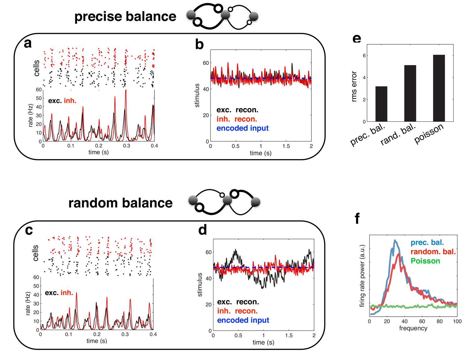
Spiking response (a), and neural reconstruction (b) of a network with heterogenous read-out weights (and connection strengths).
(c–d) Similar to panels a–b, except with randomized recurrent connections. (e) Root-mean-squared reconstruction error for each model variant, including a population of Poisson units with matching firing rates. (f) Power spectrum of population firing rate for each model variant.
Download links
A two-part list of links to download the article, or parts of the article, in various formats.
Downloads (link to download the article as PDF)
Open citations (links to open the citations from this article in various online reference manager services)
Cite this article (links to download the citations from this article in formats compatible with various reference manager tools)
Neural oscillations as a signature of efficient coding in the presence of synaptic delays
eLife 5:e13824.
https://doi.org/10.7554/eLife.13824


