Extracellular interactions and ligand degradation shape the nodal morphogen gradient
- University of Warwick, United Kingdom
- National University of Singapore, Singapore
Figures
Figure 1 with 1 supplement

Activity range and diffusion of Nodal-GFP fusion proteins.
(A) Constructs used for profiling fluorescent Nodal fusion proteins in embryos. S, signal peptide; Pro, pro-domain; Mat, mature-domain; sec-EGFP, secreted EGFP. Red arrow indicates convertase cleavage sites. (B) Injection procedure. (C) Confocal image of an injected embryo at 30% epiboly stage. White crosses mark the extracellular spots where the FCS measurements were taken. (D) Representative images of RNA in situ hybridization showing the activity range of Sqt, Cyc and mutant Nodals. Source cells are marked in brown and blue staining indicates expression of the Nodal target ntl. Scale bars, 50 μm. (E) Representative auto-correlation functions (dots) and fittings (line) of Sqt-EGFP (green) and sec-EGFP (black). (F) Table showing diffusion coefficients of the Nodal and Lefty fusion proteins as measured by FCS.
-
Figure 1—source data 1
Individual FCS measurements and diffusion coefficient values for EGFP-tagged Nodals and Leftys compared to control secreted EGFP.
- https://doi.org/10.7554/eLife.13879.004
Figure 1—figure supplement 1
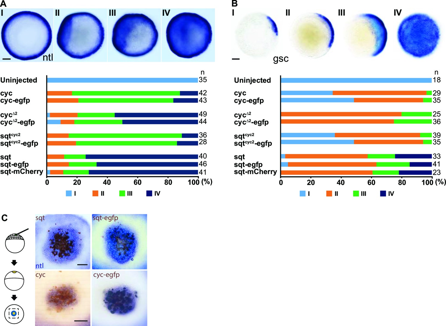
(Related to Main Figure 1).
Tagged Nodals show similar activity compared to their untagged counterparts. (A) Induction of ntl in embryos overexpressing Nodal or Nodal fusions. Five picogram aliquots of RNA was injected into one-cell stage wild-type embryos and ntl transcript expression was examined at 50% epiboly. Animal pole views of embryos showing endogenous ntl expression (I), and mild (II) or massive (III and IV) expansion of the ntl expression domain. Embryos were assessed and counted accordingly. Percentages for each class are shown in the histogram. (C) Induction of gsc in embryos overexpressing Nodal or Nodal fusions. Animal pole views of embryos showing endogenous gsc expression (I), mild expansion (II) or massive expansion (III and IV) of gsc expression domains. (C) Five picogram aliquots of RNA encoding Nodal or Nodal fusions were injected into one-cell at the 128-cell stage with a lineage tracer (Biotin-Dextran, brown color staining). Range of signaling was examined by detecting ntl transcription (blue/purple color staining). Scale bars represent 100 µm.
Figure 2
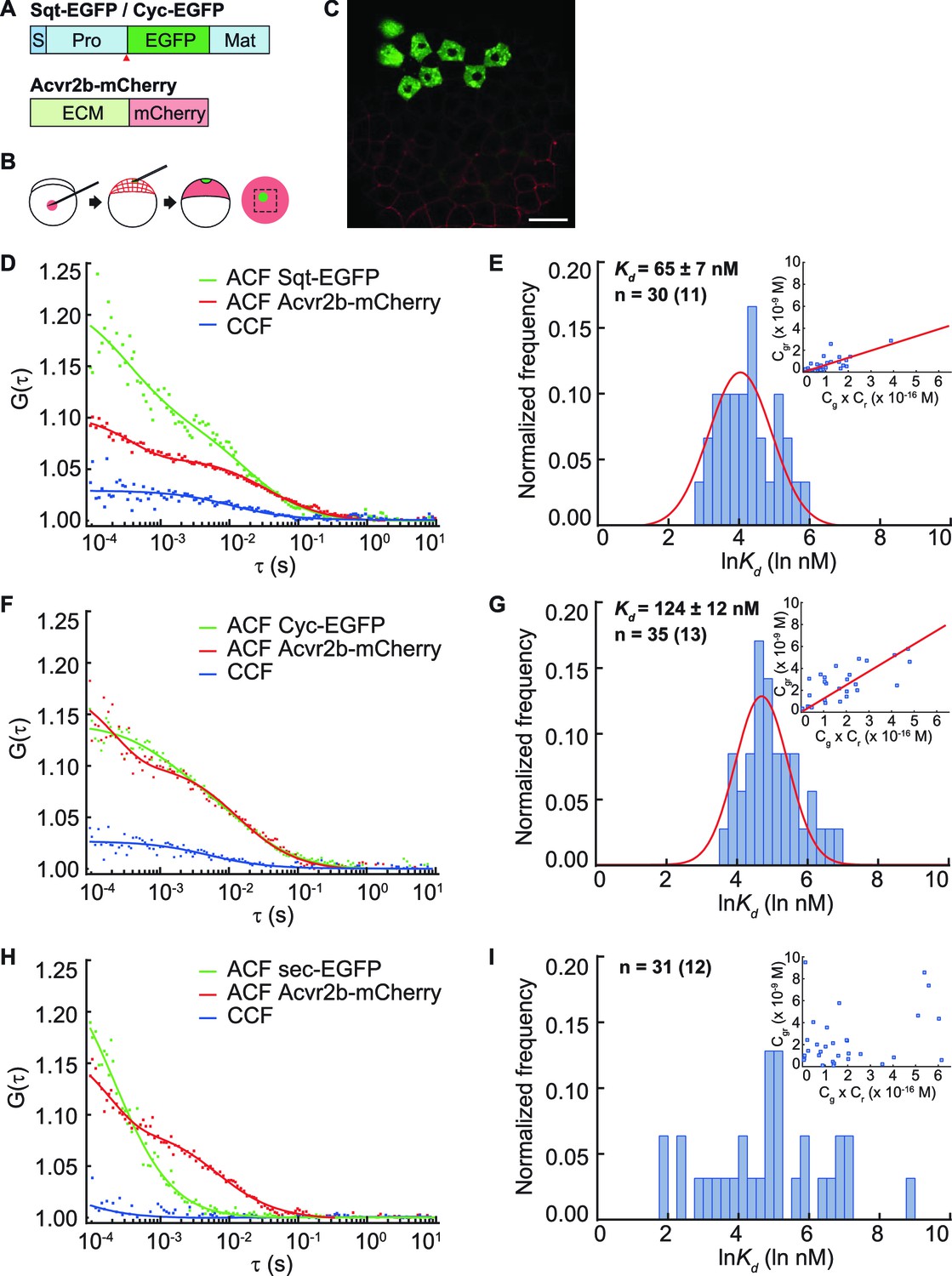
Sqt has higher affinity to the Acvr2b receptors than Cyc.
(A) Sqt-/Cyc-/sec-EGFP and Acvr2b-mCherry constructs. S, signal peptide; Pro, pro-domain; Mat, mature-domain; ECM, extracellular and transmembrane domain. Red arrows indicate convertase cleavage sites. Sqt signal peptides and pro-domain were used in sec-EGFP constructs. (B) Injection procedure. (C) Representative image of an injected embryo at 30% epiboly stage showing the expression patterns of the fusion proteins. Scale bar represents 50 μm. (D,E,F) Representative auto-correlation (ACF) and cross-correlation functions (CCF) and fits. (G,H,I) Individual Ln(Kd) frequency histogram and Gaussian fitting (red curve). Inset, concentration plot and linear regression (red line). X axis, concentration of bound protein (Cgr (x10-9 M)); Y axis, products of concentrations of free proteins (Cg x Cr (x10-16 M)). n = number of data points (number of embryos).
Figure 3
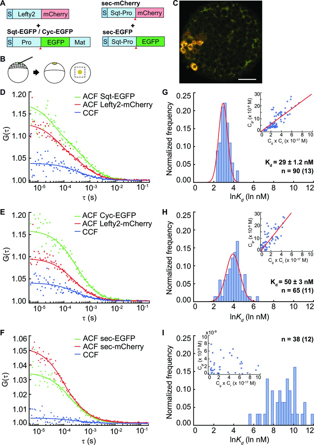
FCCS measurements reveal that Lefty has higher affinity to Sqt compared to Cyc.
(A) Constructs used for injection. S, signal peptide; Pro, pro-domain; Mat, mature-domain. Red arrows indicate the convertase cleavage sites. (B) Injection procedure. (C) Confocal image of an injected embryo at 30% epiboly showing the expression patterns of the fusion proteins. Scale bar represents 50 μm. (D, E, F) Representative auto- and cross-correlation functions (ACF; CCF) and fittings. (G, H, I) Individual Ln(Kd) frequency histogram and Gaussian fits (red curve). Inset, concentration plot and linear regression (red line). X axis, concentration of bound protein (Cgr(x10-9 M)); Y axis, products of concentrations of free proteins (Cg x Cr(x10-17 M)). n = number of data points (i.e., number of embryos).
Figure 4 with 1 supplement
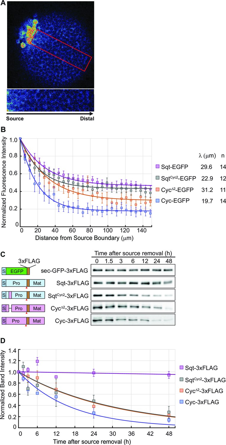
The distribution of Nodal proteins correlates with clearance.
(A) Upper, representative image and region of interest (red rectangle) for measuring distribution; lower, inset showing magnified region of interest. (B) Normalized distribution profiles and fitting. Error bars indicate standard error of mean (s.e.m). (C) Representative western blots of Nodal proteins harvested from HEK293T cell culture medium at different time points after removal of the source. The Nodal proteins were immuno-precipitated with anti-FLAG antibody and detected by western blot with the same antibody. Schematics on the left show the position of the FLAG epitope tags in each construct. (D) The profile of Nodal protein levels over time after source removal. The data points were fitted with an exponential decay model. Error bars indicate s.e.m.
-
Figure 4—source data 1
Gradient data for tagged wild type and mutant Nodals.
- https://doi.org/10.7554/eLife.13879.009
Figure 4—figure supplement 1
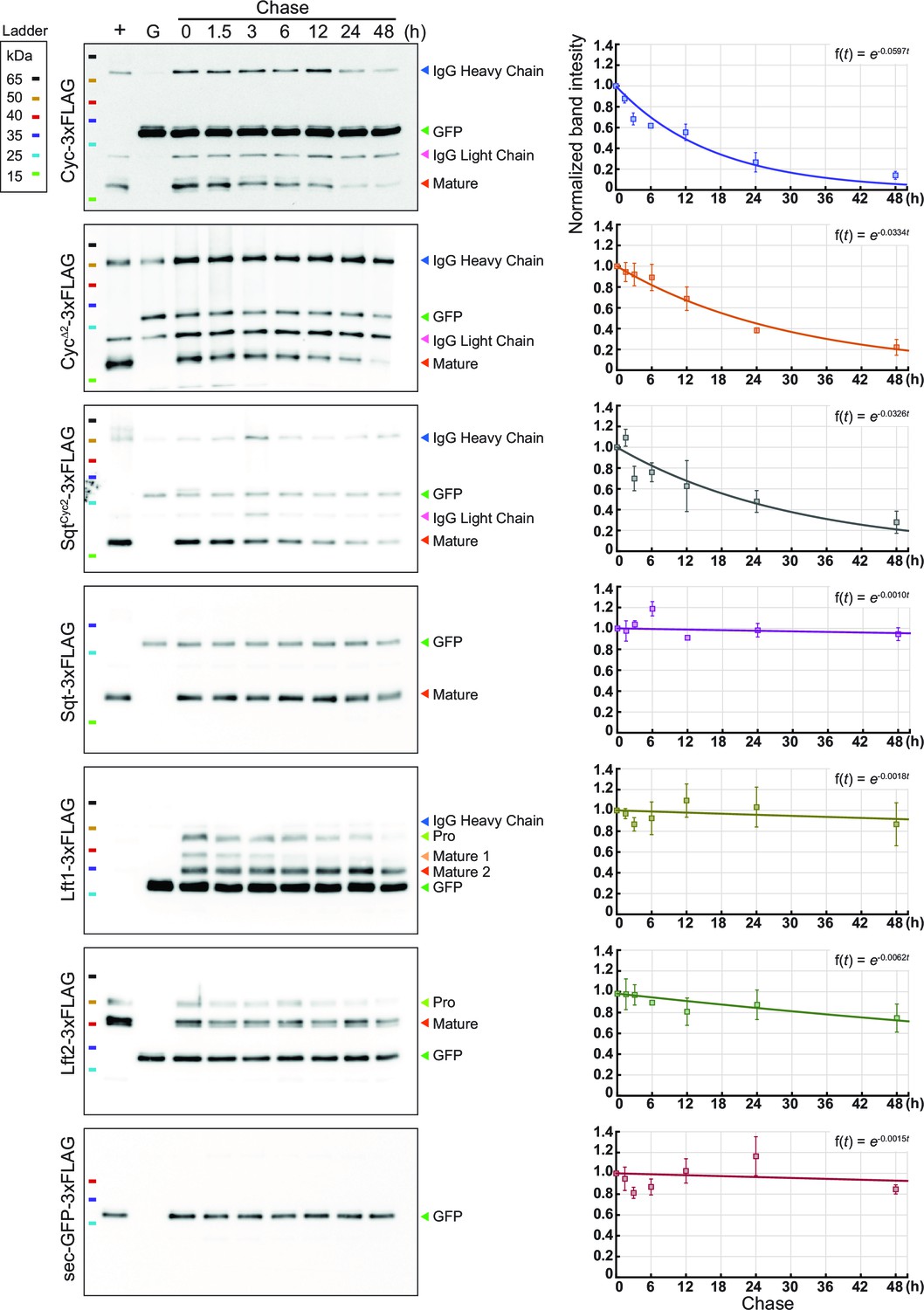
(Related to Main Figure 4).
Representative immunoblots showing protein degradation over time. Left, representative immunoblots. Equal amounts of sec-GFP-3xFLAG supernatant was added in all of the samples as input controls. Right, quantitation and fitting of protein expression levels. Each experiment was repeated three times, and the band intensity of the Nodal or Lefty proteins was normalized to GFP (input control) and to time 0 hr. The plots were then fitted with exponential decay (equation shown on the upper right corner).
Figure 5
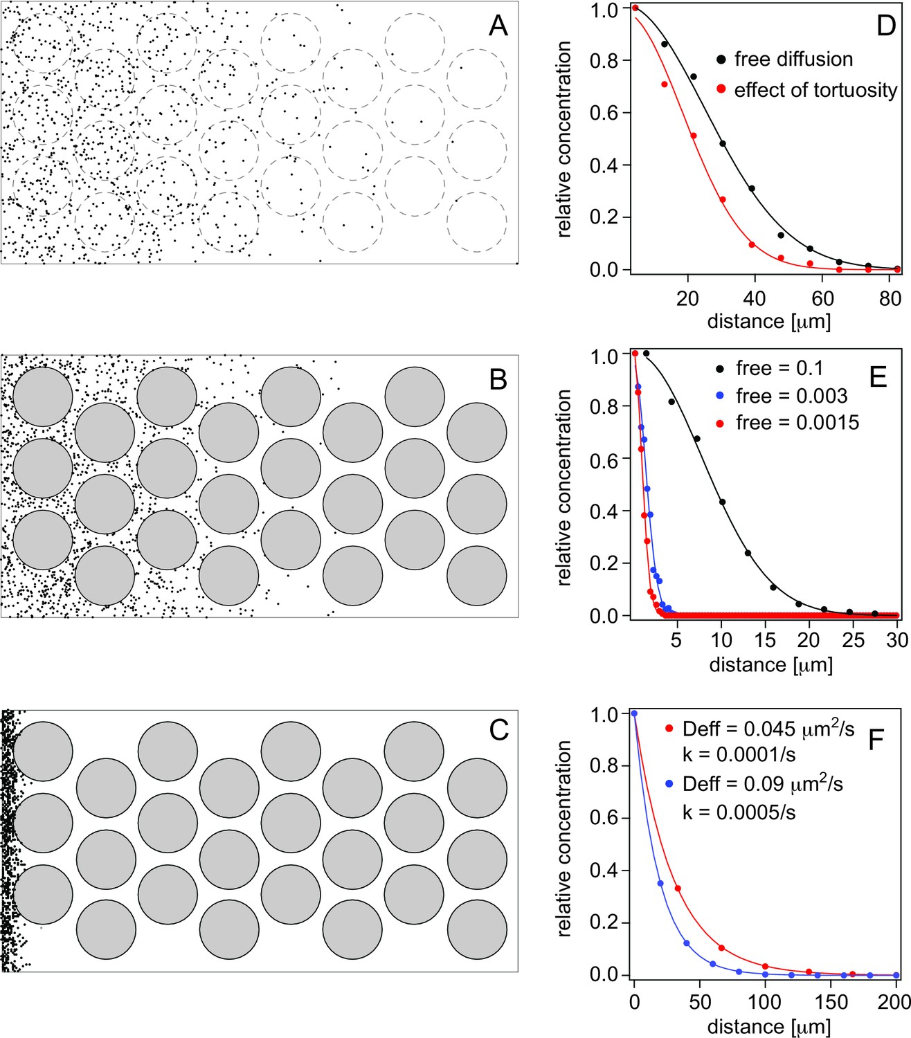
Simulations of morphogen diffusion.
(A) Free diffusion with a diffusion coefficient D = 60 μm2/s. (Dashed circles indicate positions of cells in later simulations but not taken account of in this case). (B) Diffusion in the presence of cells. (C) Diffusion in the presence of cells and binding with an average number of free particles of 0.003, i.e. 99.7% of all particles are bound on average. Simulations were done in a 3D space as described in the text and the diffusion coefficient was D = 60 μm2/s. (D) Comparison of the spread of the particles as a function of the distance from the source (the left border in panels A–C). The concentration curves were fit with a bell curve that describes the diffusion of particles from the source. For free diffusion (A) we recover a diffusion coefficient of D = 63.4 μm2/s close to the input value, and in the presence of cells (B) this reduces to an effective diffusion coefficient of Deff = 33.8 μm2/s, demonstrating the effect of tortuosity. (E) Simulations of diffusion in the presence of cells, and with different amounts of binding. The simulated diffusion coefficient was D = 60 μm2/s. The concentration curves were fit with Equation 8. The recovered effective diffusion coefficients for a fraction of free particles of 0.1, 0.003, and 0.0015 were Deff = 2.99 μm2/s, Deff = 0.09 μm2/s, and Deff = 0.042 μm2/s, respectively, demonstrating the effect of binding on the effective diffusion coefficient. (F) Gradient formation using the effective diffusion coefficients determined from graph E and degradation rates of 0.0001/s and 0.0005/s, respectively. The blue curve represents Cyc, the red curve Sqt. Although Sqt has higher binding affinity and consequently a lower free mobile fraction, its lower degradation rate ensures that Sqt has a less steep gradient. The data was fit with an exponential function yielding gradients of 19 μm for Cyc and and 30 μm for Sqt, respectively.
Videos
Video 1
Simulation of particles moving and freely diffusing from the source.
Dashed circles indicate positions of cells in later simulations (included here for illustration only, but have no influence on the simulation).
Video 2
Particle movement is hindered by cells (black circles) around which they move.
https://doi.org/10.7554/eLife.13879.014
Video 3
Particle movement is hindered further by binding.
https://doi.org/10.7554/eLife.13879.015Tables
Table 1
Simulation parameters
| Parameter | Sqt | Cyc | Reference |
|---|---|---|---|
| Kd | 60 nM | 120 nM | This work |
| Degradation rate | 0.0001/s | 0.0005/s | Estimated from Jing et al., 2006; Müller et al., 2012 |
| Ligand concentration | ~100 nM | ~100 nM | Estimated from this work |
| Receptor concentration | 40 μM | 40 μM | Estimated from this work |
| Dfree [μm2/s] | 60 | 60 | This work |
| Dtortuosity [μm2/s] | 30 | 30 | This work and Müller et al., 2013 |
| Deff [μm2/s] | 0.045 | 0.09 | This work |
Download links
A two-part list of links to download the article, or parts of the article, in various formats.
Downloads (link to download the article as PDF)
Open citations (links to open the citations from this article in various online reference manager services)
Cite this article (links to download the citations from this article in formats compatible with various reference manager tools)
Extracellular interactions and ligand degradation shape the nodal morphogen gradient
eLife 5:e13879.
https://doi.org/10.7554/eLife.13879


