Postnatal development of retrosplenial projections to the parahippocampal region of the rat
- Norwegian University for Science and Technology, Norway
Figures
Figure 1
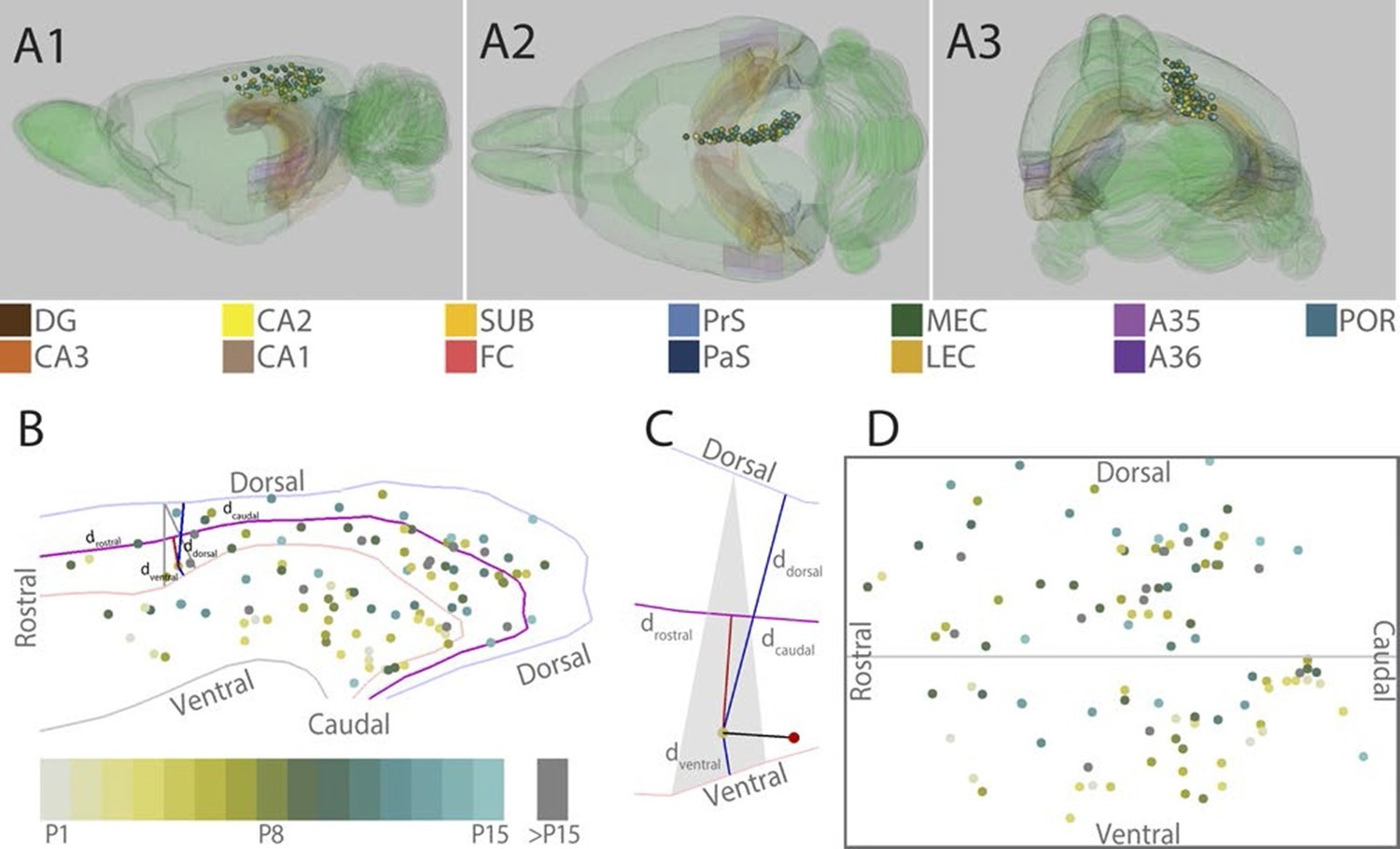
Location of the center of injections.
(A) The location of the center of each injection was normalized to a standard 3D atlas of the rat brain (Waxholm space; Papp et al., 2014; See video 1 and 2). Lateral (A1), dorsal (A2) and para-caudal view (A3) of the 3D atlas brain with the center of each injection (colored spheres). The injections are color-coded according to age (see color code bottom left). Injections were performed in either the left or right hemisphere but to ease visualization, all injections were plotted in the right hemisphere. Dentate gyrus (DG), CA3-1, subiculum (SUB), fasciola cinereum (FC), pre- and parasubiculum (PrS and PaS), medial- and lateral entorhinal cortex (MEC and LEC), A35-36 and postrhinal cortex (POR) are color coded, while the rest of the brain is colored green. (B) Midsagital view of the center of the injections projected to the pial surface. The laminar position is disregarded to allow the injections to be plotted in 2D. Light blue, light red and grey line depict respectively the dorsal border of A30, the border between A29 and A30 and the ventral border of A29. Injections are color coded according to age. Triangle explained in C. (C) One example, as shown in B, of the algorithm used for calculating normalized 2D coordinates of the injections. The pial surface area of A29 and A30 was divided into triangles (grey area). The shortest vector (black line) between the injection (red sphere) and the cortical surface was calculated. Thereafter, we calculated the coordinate of the intersection of the vector and the plane within the triangle (yellow dot) which represented the 'transposed' location of the injection. The normalized dorsoventral coordinate of each injection was defined by calculating the shortest vector from the transposed injection to dorsal () and ventral border of A29 or A30 (). The normalized rostrocaudal coordinate was obtained by first calculating a line along the rostrocaudal extend of A29 and A30, positioned equally distant from the dorsal and ventral borders (magenta line). Next, we calculated the shortest vector between the injection and this line (red line) and found the intersection between the two. The rostrocaudal coordinate was obtained by calculating the cumulative distance from the cross section to the rostral () and caudal end of RSC (). (D) Normalized flatmap of the injections. The 3D RSC is converted to a 2D normalized flatmap to obtain relative rostrocaudal and dorsoventral positions of the injections. The figure is oriented with rostral RSC (left), caudal RSC (right), dorsal RSC (top) ventral RSC (bottom) to each of the sides of the rectangle. Grey line depicts the border between A29 and A30 in RSC. In all figures, each injection is color coded according to the bottom left color scheme; light grey colored injections represent injections in pups aged P1, green colored injections represent injections in pups aged P8 while cyan colored injections represent injections in pups aged close to P15. Grey injections represent injections in pups older than P15.
Figure 2

Representative examples of injections in RSC.
(A) Normalized flatmap (see Figure 1D) of the locations of the injections in RSC, shown in B and E. Injections are located in the rostral A30 (magenta), intermediate rostral A30 (green), intermediate caudal A30 (cyan) and the intermediate rostral quarter of A29 (yellow). (B) Horizontally cut and Nissl stained section at the level of the injections overlaid with a neighboring fluorescent section containing the center of an injection in rostral A30 (magenta) and intermediate-rostral A30 (green) within the same animal. Grey line depicts delineation of A30. (C) The projections after the two injections shown in B were traced and represented in a dorsoventral series of drawings of horizontal sections through the PHR. After injections in rostral A30 (magenta) labeled fibers were mostly observed in the dorsal PrS layers I and III (C1, D1). After injections in intermediate-caudal A30 (green) the densest plexus was located more ventrally in PHR and in addition to labeled fibers in layers I, III and V-VI of PrS, labeled fibers also extended into layers V-VI of PaS, POR and MEC (C2-3 and D3). Numbers above sections indicate the dorsoventral position of the section relative to the total dorsoventral extent of PHR. The yellow boxes in C1 and C3 indicate the position of high power digital images obtained from the actual sections (D1 and D3). Grey lines depict borders between the HF-PHR subdivisions, the border between cortex and white matter and lamina dissecans. (D) High power images of plexus depicted in the sections shown in C and E. Roman numbers indicate cortical layers. Grey lines depict borders between layers. (D1) Labeled fibers in superficial layer III of PrS after injections in rostral A30 (magenta). Additionally a few fibers are seen originating in the intermediate-caudal quarter of RSC (green). (D2) Labeled fibers in proximal PrS deep layer III and layers V-VI after injection in intermediate-rostral A29 (yellow) and labeled fibers in distal PrS deep layer III and layers V-VI after injection in intermediate-caudal A30 (cyan). (D3) Labeled fibers in layers I and III after injection in intermediate-caudal A30 (green). No fibers originating in the rostral A30 were observed. (D4) After injection in intermediate-caudal A30 labeled fibers were observed in medial MEC (cyan), while after injection in intermediate-rostral A29 labeled fibers were observed in lateral MEC (yellow). (E) Top: the projections after two injections (bottom) were traced and represented in a dorsoventral series of drawings of horizontal sections through the PHR. After injections in intermediate-caudal A30 (cyan) labeled fibers were observed in distal PrS dorsally (E1-3). At more ventral levels fibers also extended into deep layers of PaS and medial MEC (E3-4). After injections in intermediate-rostral A29 (yellow) the densest plexus was located in proximal parts of PrS dorsally (E1-2). At more ventral levels the plexus in PrS layers I and III disappeared while in the deep layers the plexus shifted to lateral parts of EC at successively more ventral levels (E3-4). Numbers below sections indicate the dorsoventral position of the section relative to the total dorsoventral extent of PHR. The magenta boxes in E2 and E3 indicate the position of high power digital images obtained from the actual sections (D2 and D4). Grey lines depict borders between the HF-PHR subdivisions, the border between cortex and white matter and lamina dissecans. Bottom: Horizontally cut and Nissl stained sections at the level of the injection overlaid with neighboring fluorescent sections containing the center of an injection in intermediate-caudal A30 (cyan) and intermediate-rostral A29 (yellow) within the same animal. Gray line depicts delineation of A29 and A30. Scale bars equal 100 μm (high power images) and 1000 µm (low power images).
Figure 3
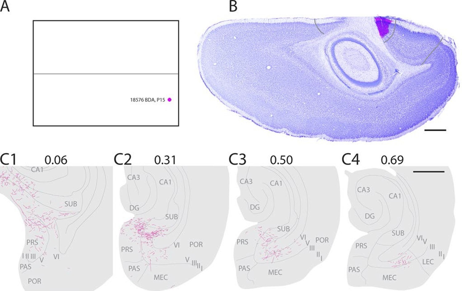
Representative example of an injection in caudal A29.
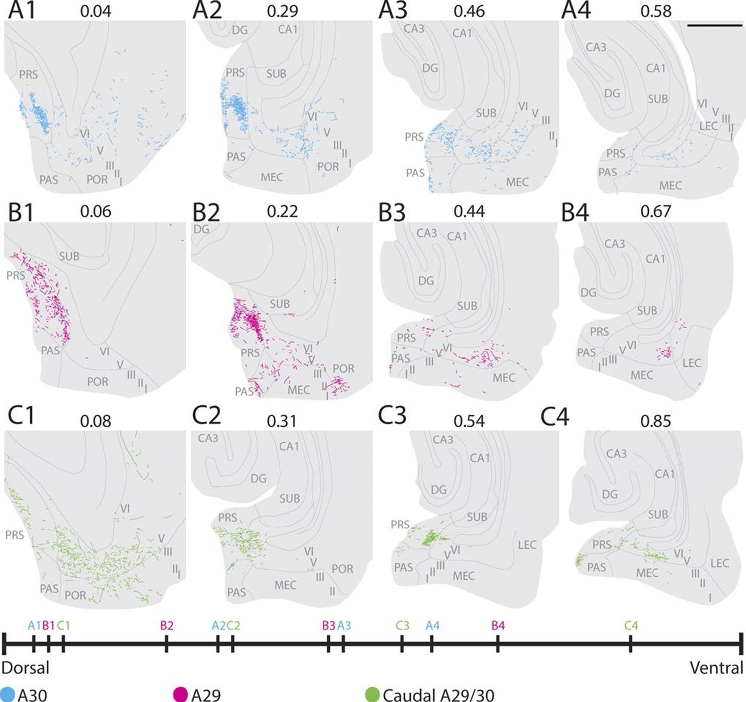
(A) Normalized flatmap with location of an injection in caudal A29 (magenta). (B) Horizontally cut and Nissl stained section at the level of the injection overlaid with an adjacent section containing the center of the fluorescent tracer injection in caudal A29 (magenta). Grey lines depict delineation of A29 and A30. (C) The projections after the injection were traced and represented in a dorsoventral series of drawings of horizontal sections through the PHR. Labeled fibers are located in more proximal parts of layers I, III and V-VI of PrS compared to after projections in A30 (compare C1-3 and Figure 2). At successively more ventral levels, fibers also extended into increasingly more lateral parts of layers V-VI of MEC compared with injections in A30 (compare C2-4 and Figure 2). Grey lines depict borders between the HF-PHR subdivisions, the border between cortex and white matter and lamina dissecans. Scale bars equal 1000 µm.
Figure 4
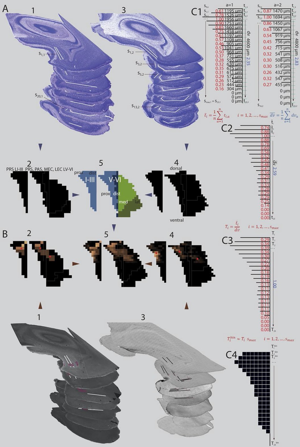
Standardized representation of location of labeled axons in PHR.
(A) Extents of PrS, deep layers of PaS and deep layers of EC were measured in the horizontal plane (1; Nissl stained sections from case 18427, 3; Nissl stained sections from case 18589). In every section, the extents of PrS, PaS, MEC and LEC along the transverse axis were measured. Based on the measurements of all sections in all brains (2 and 4) we binned the PHR along the dorsoventral and transverse axis and made an average representation of PHR (5; left: layers I and III of PrS (light blue), right: layers V-VI of PrS (light blue), PaS (dark blue), MEC (light green) and LEC (dark green). Dorsal, ventral, proximal (prox), distal (dist), medial (med), lateral (lat) indicates dorsoventral and transverse axis of the flatmaps. s#,a refers to individual measurements of layers I and III of PrS in C1. (B) Locations of labeled fibers were obtained by measuring the distance between the plexus and the borders of the field in which the plexus was located (1; case 18427, note that we inserted magenta labeled structures to illustrate labeled fibers and their respective positions on the flatmaps). The measurements were performed in every section containing a plexus. The bins between the boundaries of each plexus were given a value ranging from 1 to 3 reflecting weak to dense labeling respectively (color coded in 2, 1 = brown; 2 = orange; 3 = bright yellow). Bins outside the plexus boundaries were given the value 0 (black, no plexus). In experiments in which we observed single labeled axons or a sparse plexus, we measured the distance from each labeled axon to one of the borders of the field in which the plexus was located (3; case 18589; repeating patterns in top sections are artefacts due to stitching of digitized images). We inserted magenta labeled fibers and their respective positions on the flatmaps). We gave each bin in the flatmap a value corresponding to the number of labeled single axons (4; bins not containing any labeled fibers: black; bins with the highest number of labeled axons: bright yellow). For all flatmaps, the centers of mass for layers I and III in PrS, layers V-VI of PrS and PaS combined and layers V-VI of MEC and LEC combined were calculated (red dots). To compare groups of injections, flatmaps of individual injections were normalized to the highest valued bin, transformed to the average flatmap and added together (5; see methods for further details). (C) Binning of layers I and III of PrS along the dorsoventral and along the transverse axis. The example is based on animals 18427 (left) and 18589 (right; both shown Figure 4A and B). All subdivisions are binned according to the same algorithm. First the transverse measurements (s#,a, visualized by black lines in C1) and the dorsoventral measurement () in all sections in all animals were normalized to the longest measurement of the respective subdivision in the particular animal (red (transverse) and blue (dorsoventral) numbers in C1). Next, we binned the dorsoventral axis of each PHR subdivision (represented by turquois lines in C1) in the same amounts of bins as the maximum number of sections containing PHR in a single series (; 23 in the example) and calculated the transverse extends of each row of bins in each animal (, numbers not shown). Thereafter, we calculated the means of the normalized transverse measurements across all animals for each bin (, red numbers in C2), and the mean across all animals of the normalized dorsoventral extend of PHR (; blue number in C2). The ratio of the mean transverse extends and the mean dorsoventral extend was calculated such that each dorsoventral level was expressed as a value relative to the dorsoventral extent of PHR (; red numbers in C3). Finally, the number of bins along the transverse axis for each dorsoventral level () was calculated (C4).
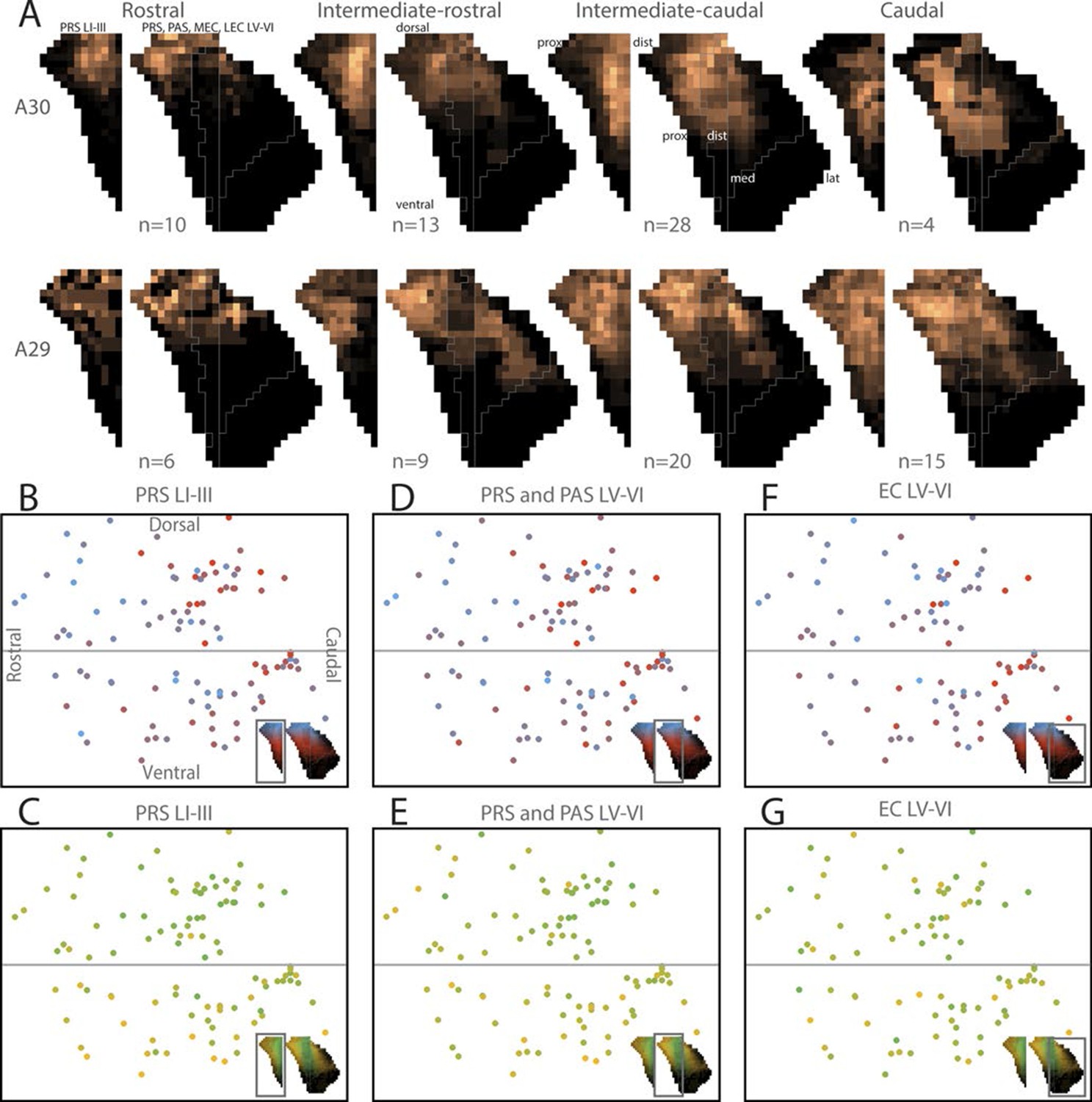
Figure 5 with 1 supplement

Topographical organization of projections.
The position of the centers of mass of labelling in layers I and III of PrS, layers V-VI of PrS and PaS and layers V-VI of MEC and LEC is plotted. Each dot is color coded with respect to the rostrocaudal (A) or dorsoventral position (B) of the injections in RSC (rostral half; blue, caudal half; red, A29; yellow, A30; green). In layers I and III of PrS more caudally placed injections result in projections located more ventral compared to rostrally placed injections (A; p<0.001), while ventrally placed injections result in projections located more proximal compared to dorsally placed injections (B; p<0.001). In layers V-VI of PrS and PaS caudally placed injections result in projections located more ventral compared with rostrally placed injections (A; p<0.001), while ventral and rostrally placed injections result in projections located significantly more proximal compared with dorsally and caudally placed injections (B; ventral: p<0.001, caudal: p=0.033). In MEC and LEC layers V-VI, caudal and ventrally placed injections result in projections located significantly more ventral compared to rostral and dorsally placed injections (A; caudal: p<0.001, ventral: p=0.032), while ventrally placed injections result in projections located significantly more lateral compared to dorsally placed injections (B; p=0.020). Multiple regression was used for all statistical tests (Figure 5—source data 1–12). For flatmaps of the projection patterns see Figure 5—figure supplement 1.
-
Figure 5—source data 1
Datapoints used in multiple regressions.
- https://doi.org/10.7554/eLife.13925.010
-
Figure 5—source data 2
Datapoints used in multiple regressions.
- https://doi.org/10.7554/eLife.13925.011
-
Figure 5—source data 3
Datapoints used in multiple regressions.
- https://doi.org/10.7554/eLife.13925.012
-
Figure 5—source data 4
Datapoints used in multiple regressions.
- https://doi.org/10.7554/eLife.13925.013
-
Figure 5—source data 5
Datapoints used in multiple regressions.
- https://doi.org/10.7554/eLife.13925.014
-
Figure 5—source data 6
Datapoints used in multiple regressions.
- https://doi.org/10.7554/eLife.13925.015
-
Figure 5—source data 7
Datapoints used in multiple regressions.
- https://doi.org/10.7554/eLife.13925.016
-
Figure 5—source data 8
Datapoints used in multiple regressions.
- https://doi.org/10.7554/eLife.13925.017
-
Figure 5—source data 9
Datapoints used in multiple regressions.
- https://doi.org/10.7554/eLife.13925.018
-
Figure 5—source data 10
Datapoints used in multiple regressions.
- https://doi.org/10.7554/eLife.13925.019
-
Figure 5—source data 11
Datapoints used in multiple regressions.
- https://doi.org/10.7554/eLife.13925.020
-
Figure 5—source data 12
Datapoints used in multiple regressions.
- https://doi.org/10.7554/eLife.13925.021
Figure 5—figure supplement 1
Topographical organization of RSC-PHR projections in pups.
(A) Injections were organized into 2 x 4 groups (A29/A30 x rostrocaudal) based on the location of the injection and the average projection pattern for each group was calculated. Injections in rostral RSC (left column) resulted in labeled fibers within dorsal PrS layers I, III and V-VI, while more caudal injections (the three right columns) resulted in labeling in more ventral parts of PrS, PaS and MEC. Injections in A30 (top row) resulted in labeled fibers in distal PrS, PaS and medial MEC. In contrast, injections in A29 (bottom row) resulted in labeled fibers in more proximal parts of PrS and more lateral parts of MEC. Dorsal, ventral, proximal (prox), distal (dist), medial (med), lateral (lat) indicates dorsoventral and transverse axis of the flatmaps. (B-G) Centers of mass of the labeling resulting from each injection were calculated for PrS layers I and III (B and C), PrS and PaS layers V-VI (D and E) and MEC and LEC layers V-VI (F and G). In the plots, each injection is plotted according to its location in RSC and colorcoded according to the dorsal (blue), ventral (red), distal/medial (green) and proximal/lateral (yellow) position of the center of mass of the projection in PHR (see color maps in bottom right of each figure).
Figure 6 with 2 supplements
Development of topographies.
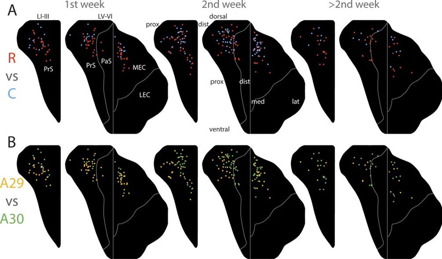
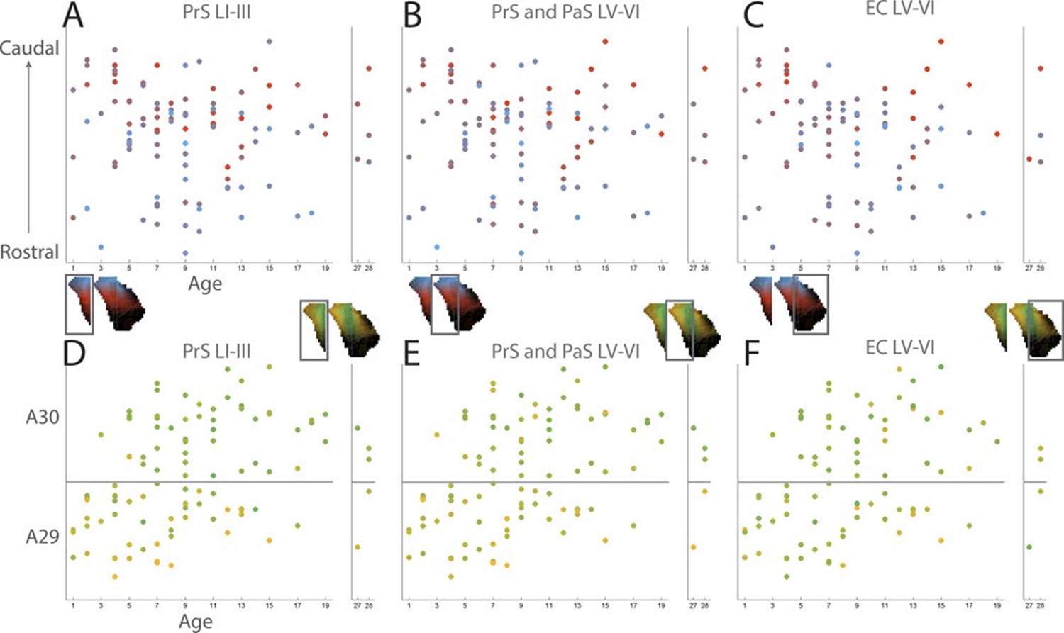
The position of the centers of mass of the labelling in layers I and III of PrS, layers V-VI of PrS and PaS and layers V-VI of MEC and LEC is plotted (see also Figure 6—figure supplement 2). Each dot is color coded with respect to the rostrocaudal (A) or dorsoventral position (B) of the injections in RSC (rostral half; blue, caudal half; red, A29; yellow, A30; green). Left column; animals aged P1-6, middle column; animals aged P7-13, right column; animals aged P14-28. Age is not related to the dorsoventral position of the plexus (PrS LI-III: p=0.876; PRS and PaS LV-VI; p=0.187; EC LV-VI: p=0.198) or the transverse position of the plexus (PrS LI-III: p=0.641; PrS and PaS LV-VI; p=0.325; EC LV-VI: p=0.402). Multiple regression was used for all statistical tests (Figure 5—source data 1–12). For flatmaps of the projection patterns see Figure 6—figure supplement 1.
Figure 6—figure supplement 1
Flatmaps of projection patterns of different age groups.
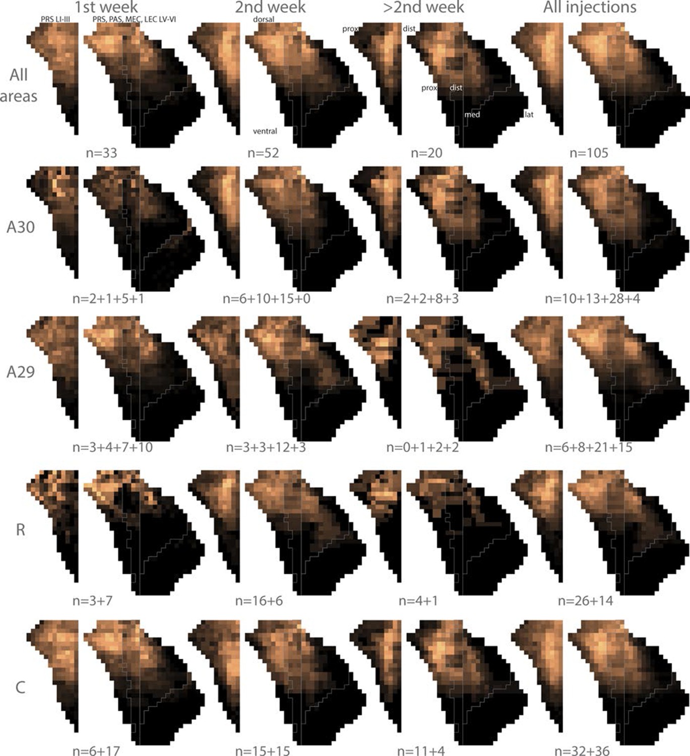
All injections were subdivided into three groups based on the age of the injected animal. 1st column shows flatmaps of averaged labeling patterns in animals injected during the 1st postnatal week, 2nd column shows flatmaps of animals injected during the 2nd postnatal week, 3rd column shows flatmaps of animals injected during the 3rd postnatal week or later and the 4th column contains animals across all ages. The 1st row shows flatmaps of labeling patterns independent of the location of the injection. Numbers under the flatmap depict the number of experiments in each group. The 2nd row shows flatmaps of the labeling patterns observed after injections in A30, while the 3rd row shows flatmaps of the labeling patterns observed after injections in A29. In row 3 and 4 the numbers under the flatmap depict the number of injections in rostral quarter of RSC + the number of injections in the intermediate-rostral quarter of RSC + the number of injections in the intermediate-caudal quarter of RSC + the number of injections in the caudal quarter of RSC. The 4th row shows flatmaps of the labeling pattern observed after injections in the rostral half (R) of RSC while the 5th row shows injections in the caudal half (C) of RSC. In rows 4 and 5 the numbers under the flatmap depict the number of injections in A29 + the number of injections in A30 in the respective group. Dorsal, ventral, proximal (prox), distal (dist), medial (med), lateral (lat) indicates dorsoventral and transverse axis of the flatmaps.
Figure 6—figure supplement 2
Development of topographies.
(A–C) Centers of mass of the labeled plexus after each injection were calculated for PrS layers I and III (A), PrS and PaS layers V-VI (B) and MEC and LEC layers V-VI (C). In the plots each injection is plotted according to the age of the animal and the rostrocaudal position in RSC and color coded according to the dorsal (blue), ventral (red) position of the center of mass of the projection in PHR (see color maps in bottom left of each figure). (D–F) Centers of mass of the labeled plexus after each injection were calculated for PrS layers I and III (D), PrS and PaS layers V-VI (E) and MEC and LEC layers V-VI (F). In the plots each injection is plotted according to the age of the animal and the dorsoventral position in RSC and color coded according to the proximal/lateral (yellow) and distal/medial (green) position of the center of mass of the projection in PHR (see color maps in top right of each figure).
Figure 7
Labelling patterns in the adult.
(A) An injection in intermediate rostrocaudal A30 resulted in dense labelling in layers I and III of distal PrS and a few fibers in deep PrS, PaS and POR (A1). More ventrally, fibers also invaded the MEC with the most fibers located medially in MEC (A3). (B) An injection in intermediate rostrocaudal A29 resulted in a dense fiber plexus in layers I and III of proximal PrS and POR (B2). At this dorsoventral level a few fibers also invaded PaS. More ventrally, a fiber plexus was present in lateral MEC. (C) An injection at the border of A29 and A30 in caudal RSC resulted in fibers located in layer I of PrS and deep PaS and POR dorsally (C1). More ventrally, a dense projection to layers I and III of PrS (C2 and 3) and a moderate projection to intermediate mediolateral MEC was present (C4). In A-C numbers above each section depict normalized dorsoventral position of the section and the line at the bottom of the figure represents the relative dorsoventral position of each section. Scale bar equals 1000 µm.
Figure 8
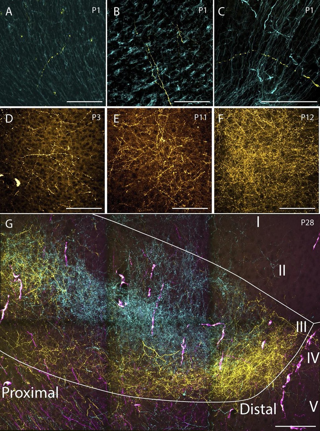
Examples of the densest fiber plexus observed in PHR at different ages.
At birth, single unbranching fibers were present in superficial layers of PrS (A), deep layers of PrS (B) and deep layers of MEC (C). At P3, some branching fibers were observed (D, PrS). These fibers typically branched only once or twice. At P11 (E, PrS) the complexity of the fiber plexus increased as fibers have multiple branching points and thin fibers are seen within the plexus. At P12 (F, PrS) the first plexus which was comparable to plexus in adolescent animals (G, PrS) and adults (data not shown) was observed. In the experiment shown in G, the terminal distribution of three differentially labeled projections is illustrated. A plexus resulting from an injection in intermediate-rostral A29 (yellow) terminated throughout layer III of PrS, while the plexus observed after an injection in intermediate-rostral A30 terminated in the center of layer III of PrS (cyan). Fibers originating from a third injections in intermediate-caudal RSC (magenta) are observed, however the densest fiber plexus is located in a section at more ventral levels of PrS. The large, overlapping magenta and yellow structures are endothelium which take up alexa-preconjugated dextran amines. White line depicts the deep and superficial borders of layer III. Scale bars equal 100 μm.
Figure 9

RSC projections to PHR arise from neurons in layer V.
(A) A FB injection in deep layers of mainly PrS and PaS (top right; P5, coronal section) resulted in retrograde labeling of neurons in CA1, SUB and RSC (top row). Coronal sections shown are from intermediate-rostral RSC (1), intermediate-caudal RSC (2) and caudal RSC (3). Cyan squares depict size and position of high-power images in the bottom row. Bottom row: High power images of retrogradely labeled neurons in superficial layer V of RSC. Dashed lines depict the pia and the border between cortex, white matter and the corpus callosum. Solid lines depict borders between layer I, layers II-III and layer V and border between A29 and A30. Scale bars equal 100 μm (high power images) and 1000 µm (low power images). (B) FB was injected in an intermediate dorsoventral level in MEC and PaS (top right; P11, horizontal sections) and resulted in retrogradely labeled neurons in superficial layer V of caudal RSC (top row). Horizontal sections are organized from dorsal (1) to ventral (3). Cyan squares depict location of high-power images in the bottom row. White lines depicts borders of RSC and border between A29 and A30. Bottom row: High power images of retrogradely labeled neurons in superficial layer V of RSC. Dashed lines depict the pia and the border between cortex and white matter. Solid lines depict borders between layer I, layers II-III and layer V. Scale bars equal 100 μm (high power images) and 1000 µm (low power images).
Figure 10
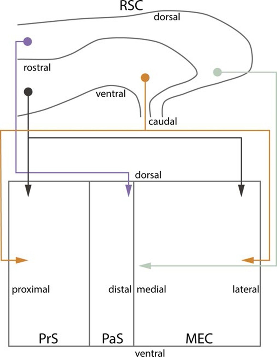
Summary of topographical organization of projections from RSC to PHR in the developing and adult brain.
Schematic representation of the organization of the projections from RSC (top) to PHR (bottom). Projections from RSC to PHR terminate mainly in PrS, PaS and MEC. Projections originating from rostral RSC (purple and black) terminate in dorsal PHR, while projections originating from caudal RSC (yellow and grey) terminate in more ventral parts of PHR. Projections originating from ventral RSC (black and yellow) terminate in proximal PrS and in lateral parts of MEC, while projections originating from dorsal RSC (purple and grey) terminate in distal PrS and in medial parts of MEC.
Videos
Video 1
Representation of all injection sites in RSC represented in a 3D rendering of the rat brain (Waxholm space; Papp et al., 2014; 2015).
The injection sites are color coded for age (for code see Figure 1)
Video 2
Representation of all injection sites in RSC represented in a 3D rendering of the rat brain (Waxholm space; Papp et al., 2014; 2015).
The injection sites are color coded for age (for code see Figure 1)
Download links
A two-part list of links to download the article, or parts of the article, in various formats.
Downloads (link to download the article as PDF)
Open citations (links to open the citations from this article in various online reference manager services)
Cite this article (links to download the citations from this article in formats compatible with various reference manager tools)
Postnatal development of retrosplenial projections to the parahippocampal region of the rat
eLife 5:e13925.
https://doi.org/10.7554/eLife.13925


