Adaptation in protein fitness landscapes is facilitated by indirect paths
- University of California, Los Angeles, United States
Figures
Figure 1 with 6 supplements
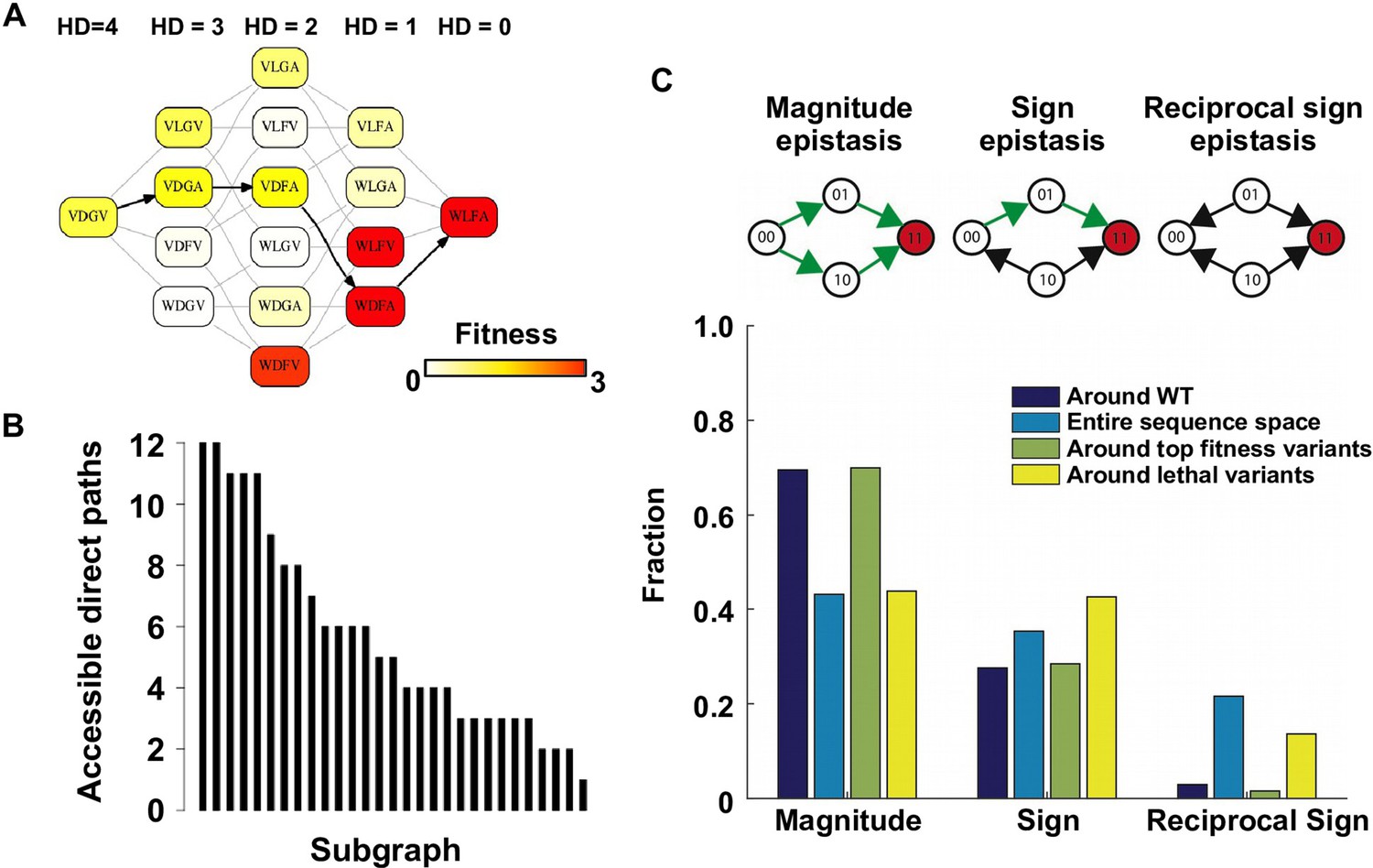
Direct paths of adaptation are constrained by pairwise epistasis.
(A) An example of subgraph that contains VDGV (wild type, WT), the quadruple mutant WLFA and all intermediates between them. Each variant in the subgraph is represented by a node. Edges are drawn between nearest neighbors. The arrows in bold represent the only accessible direct path of adaptation from VDGV to WLFA. HD: Hamming distance. (B) We identified a total of 29 subgraphs in which the quadruple mutant was the only fitness peak. The number of accessible direct paths from WT to the quadruple mutant is shown for each subgraph. The maximum number of direct paths is 24. (C) The fraction of three types of pairwise epistasis around WT (2091 out of 2166), randomly sampled from the entire sequence space (105 in total), or in the neighborhood of the top 100 fitness variants and 100 lethal variants. We note that this analysis is different from previous studies on how epistasis changes along adaptive walks, where the quadruples are chosen such that the fitness values of genotype 00, 01 and 11 are in increasing order (Greene and Crona, 2014). Sign epistasis and reciprocal sign epistasis, both of which can block adaptive paths, are prevalent in the fitness landscape. Classification scheme of epistasis is shown at the top. Each node represents a genotype, which is within a sequence space of two loci and two alleles. Green arrows represent the accessible paths from genotype “00” to a beneficial double mutant “11” (colored in red).
Figure 1—figure supplement 1
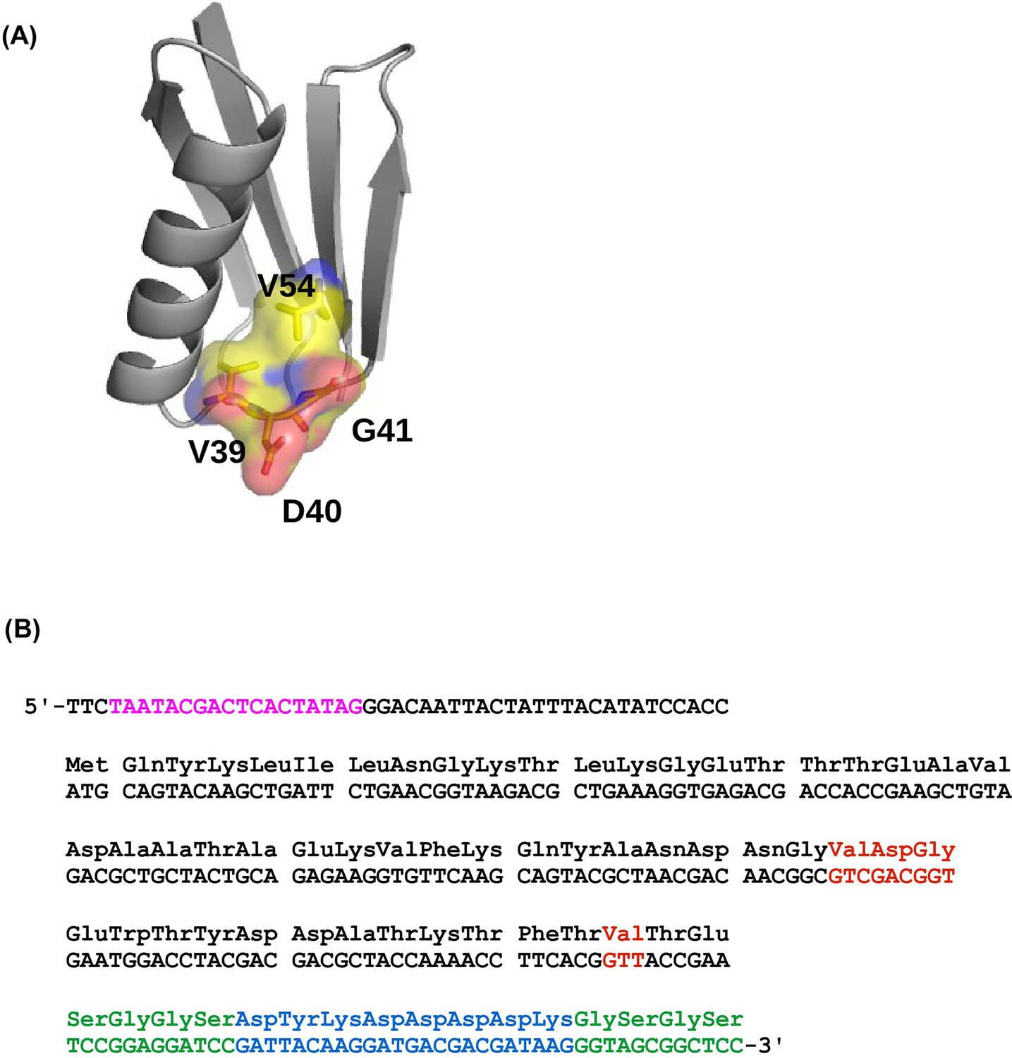
The four-site sequence space of protein G.
(A) The locations of sites 39, 40, 41, and 54 of protein GB1 are shown on the protein structure. PDB: 1PGA (Gallagher et al., 1994). (B) The WT sequence of the nucleotide template (Olson et al., 2014). T7 promoter is highlighted in magenta. Randomized sites (39, 40, 41, and 54) are highlighted in red. Poly-GS linkers are highlighted in green. FLAG-tag is highlighted in blue.
Figure 1—figure supplement 2
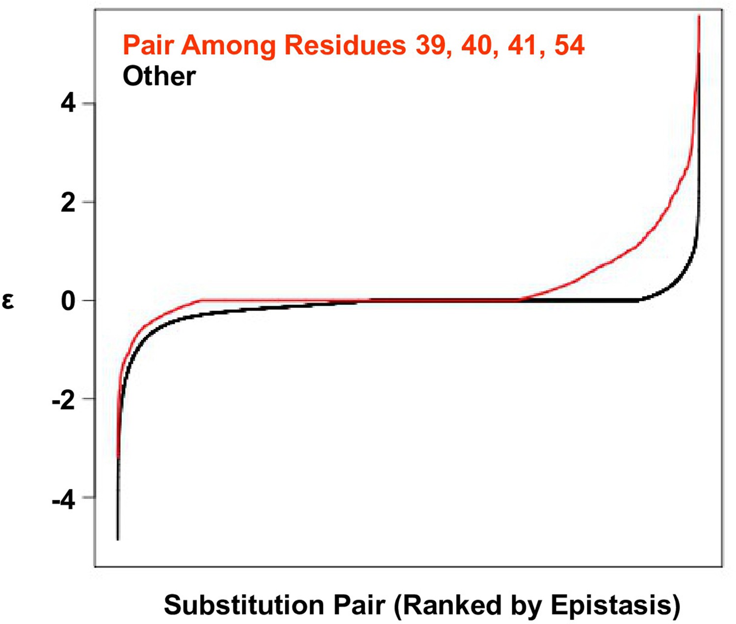
Positive epistasis is enriched in the four-site sequence space.
The distribution of pairwise epistasis measured by Olson et al. (Olson et al., 2014). The pairwise epistatic values among sites 39, 40, 41, and 54 are ranked and represented by the red line. The pairwise epistatic values among other sites (all but 39, 40, 41, and 54) are ranked and represented by the black line.
Figure 1—figure supplement 3
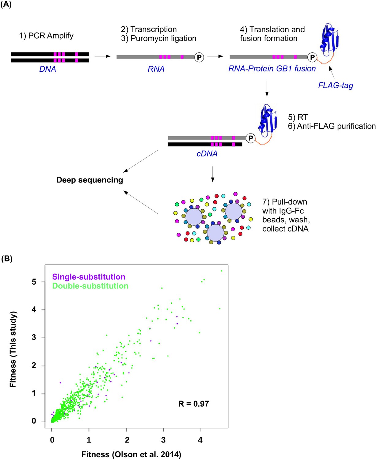
Workflow of mRNA display and data validation.
(A) The workflow of mRNA display is shown. This is adapted from (Olson et al., 2014). (B) The fitness values for all single substitution variants and double substitution variants in this study and in our previous study (based on an independently constructed library) (Olson et al., 2014) are compared. The high correlation (Pearson correlation = 0.97, p<2.2× 10⁻¹⁶) validates the fitness data obtained in this study.
Figure 1—figure supplement 4
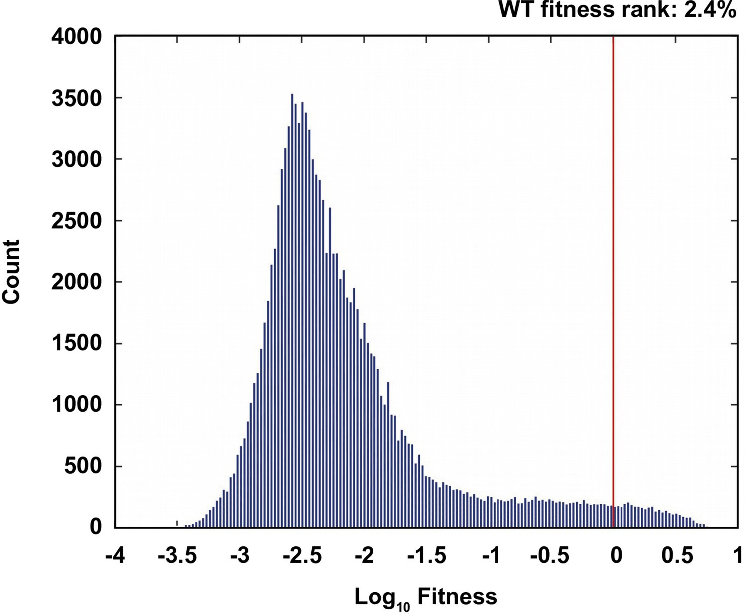
Comparison of the wild type to the ensemble of possible genotypes.
(A) The distribution of fitness values of all non-lethal genotypes. The fitness rank of the wild type genotype is 2.4% in the distribution of all fitness measurements. 19.7% of the measured genotypes are lethal (fitness=0).
Figure 1—figure supplement 5
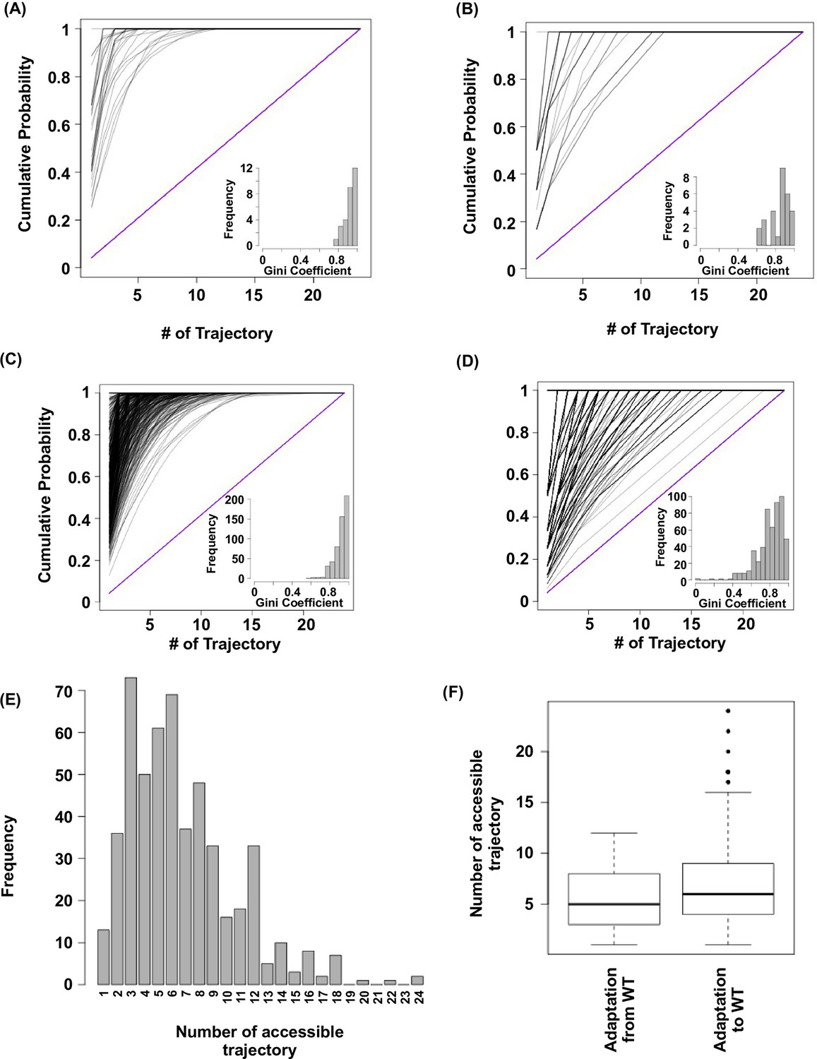
Subgraph analysis.
We calculated the relative probabilities to realize each accessible path (Weinreich et al., 2006) (see Materials and methods). In all the subgraphs analyzed, we found that most of the realizations were captured by a few accessible paths, as demonstrated by the skew in the cumulative probability of realization among different paths. (A) Cumulative probability of realization for mutational trajectories from WT (VDGV) to beneficial variants that have a Hamming distance (HD) of 4 from WT. This analysis only included those subgraphs with a reachable quadruple mutation variant (HD = 4 from WT) as the only fitness peak. Correlated Fixation Model is used. The diagonal line indicates the cumulative probability of a subgraph with equal probability of realization for all 24 possible trajectories. The bias of probability of realization in each subgraph was quantified using the Gini index (see Materials and methods) and is shown as a histogram in the inset. (B) Same as panel A, except Equal Fixation Model is used instead. (C and D) Cumulative probability for mutational trajectories from a deleterious variants that have a Hamming distance (HD) of 4 from WT (VDGV) to WT. This analysis only included those subgraphs with WT being the only fitness peak and the quadruple variant has a fitness between 0.01 to 1. The diagonal line indicates the cumulative probability of a subgraph with equal probability of realization for all 24 possible trajectories. The bias of probability of realization in each subgraph was quantified using the Gini index and is shown as a histogram in the inset. A total of 526 subgraphs were analyzed. (C) Correlated Fixation Model is used. (D) Equal Fixation Model is used. (E) Number of accessible trajectory from a deleterious variants that have a Hamming distance (HD) of 4 from WT (VDGV) to WT in each subgraph is shown as a barplot. The maximum possible number of accessible trajectory is 24. (F) The distribution of number of accessible trajectory is shown as a box plot. “Adaptation from WT” indicates those subgraphs based on the adaptation from WT to a beneficial variant that has a Hamming distance of 4 from WT. “Adaptation to WT” indicates those subgraphs based on the adaptation from a deleterious variant that has a Hamming distance of 4 from WT to WT.
Figure 1—figure supplement 6
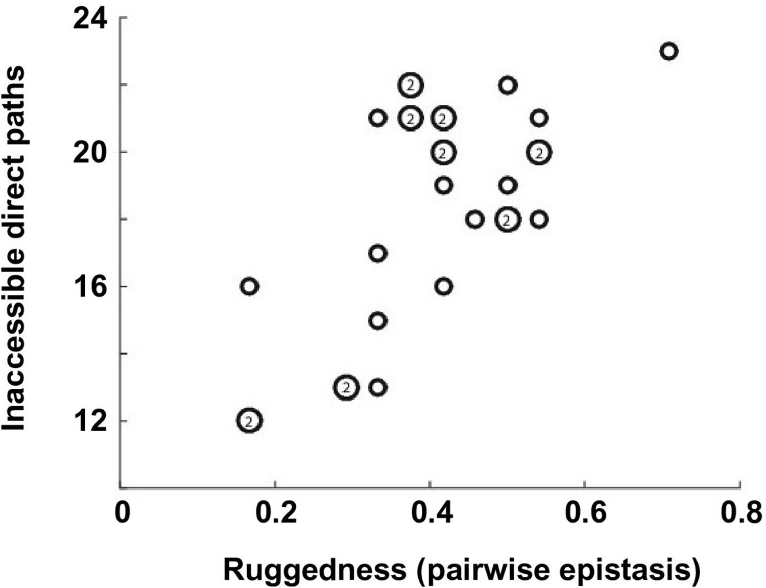
Correlation between the number of selectively inaccessible direct paths and ruggedness.
The number of inaccessible direct paths is positively correlated (Pearson correlation = 0.66, p=1.0 × 10⁻⁴) with the ruggedness induced by sign and reciprocal sign epistasis. The level of ruggedness is quantified as , where denotes the fraction of each type of pairwise epistasis. The number inside a symbol indicates the number of subgraphs with identical properties.
Figure 2 with 1 supplement
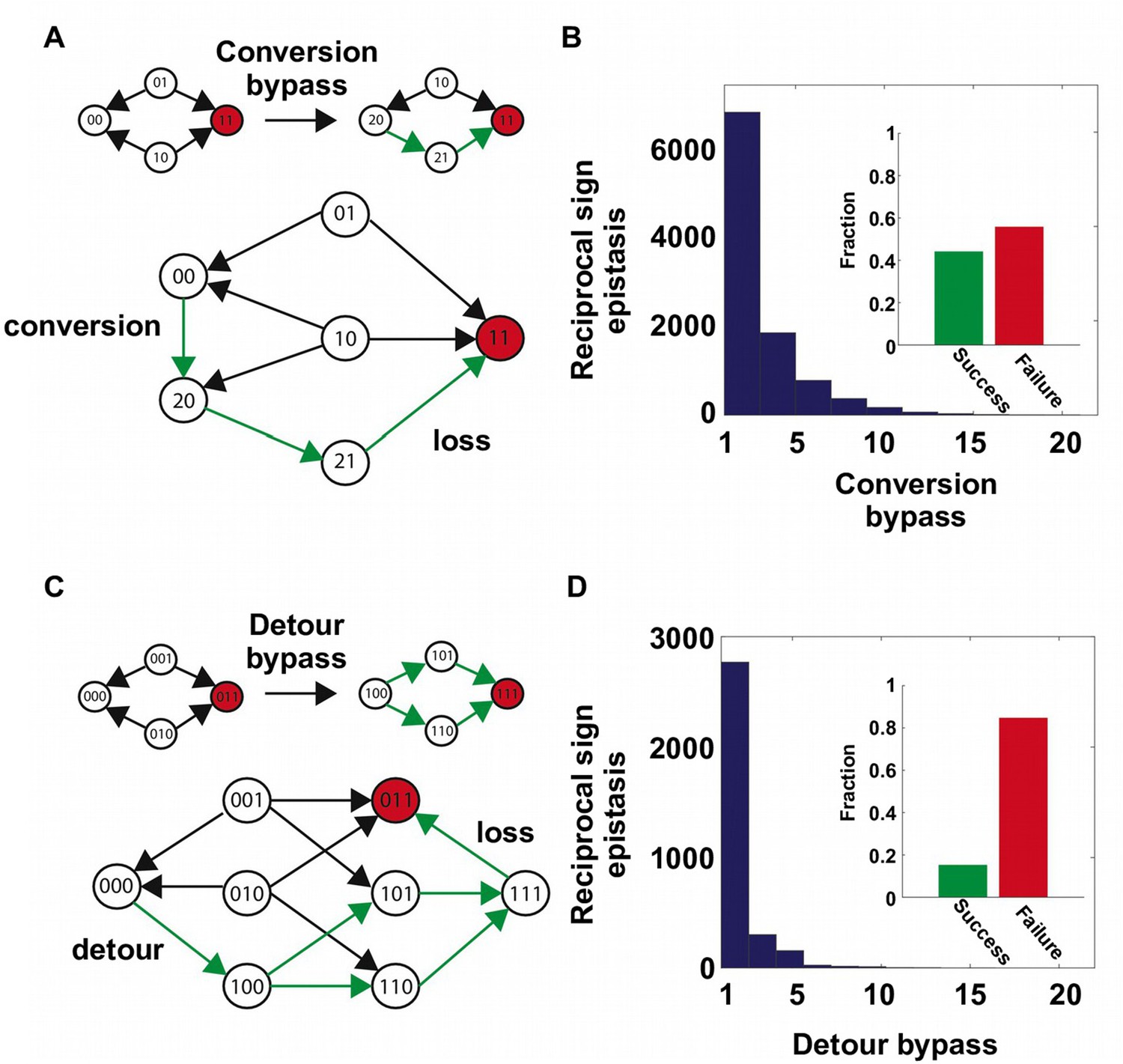
Two distinct mechanisms of extra-dimensional bypass.
(A) Extra amino acids at one of the two interacting sites may open up potential paths that circumvent the reciprocal sign epistasis. The starting point is 00 and the destination is 11 (in red). Green arrows indicate the accessible path. A successful bypass would require a “conversion” step that substitutes one of the two interacting sites with an extra amino acid (), followed by the loss of this mutation later (). The original reciprocal sign epistasis is changed to sign epistasis on the new genetic background after conversion. (B) Among ~20,000 randomly sampled reciprocal sign epistasis, >40% of them can be circumvented by at least one conversion bypass (i.e. success, inset). The number of available bypass for the success cases is shown as histogram. (C) The second mechanism of bypass involves an additional site. In this case, adaptation involves a “detour” step to gain mutation at the third site (), followed by the loss of this mutation (). The original reciprocal sign epistasis is changed to either magnitude epistasis or sign epistasis on the new genetic background after detour (Figure 2—figure supplement 1). (D) In comparison to conversion bypass, detour bypass has a lower probability of success (<20%, inset) and is less prevalent.
Figure 2—figure supplement 1
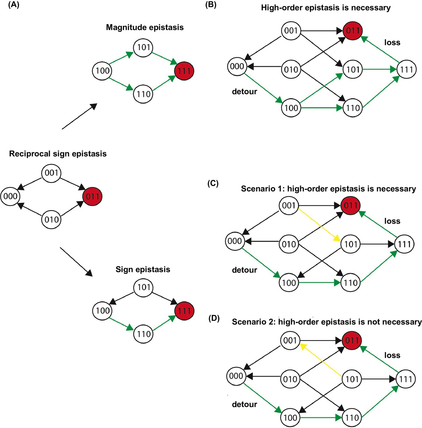
Three scenarios of extra-dimensional bypass via an extra site.
(A) Reciprocal sign epistasis may be bypassed via the involvement of a third site. (B–D) There are three possible scenarios. With a mutation at the third site, reciprocal sign epistasis between the first two sites can be changed to magnitude epistasis in (B) or sign epistasis in (C–D). It can be proven that higher-order epistasis is required for the scenarios in (B) and (C) (see Materials and methods).
Figure 3 with 6 supplements
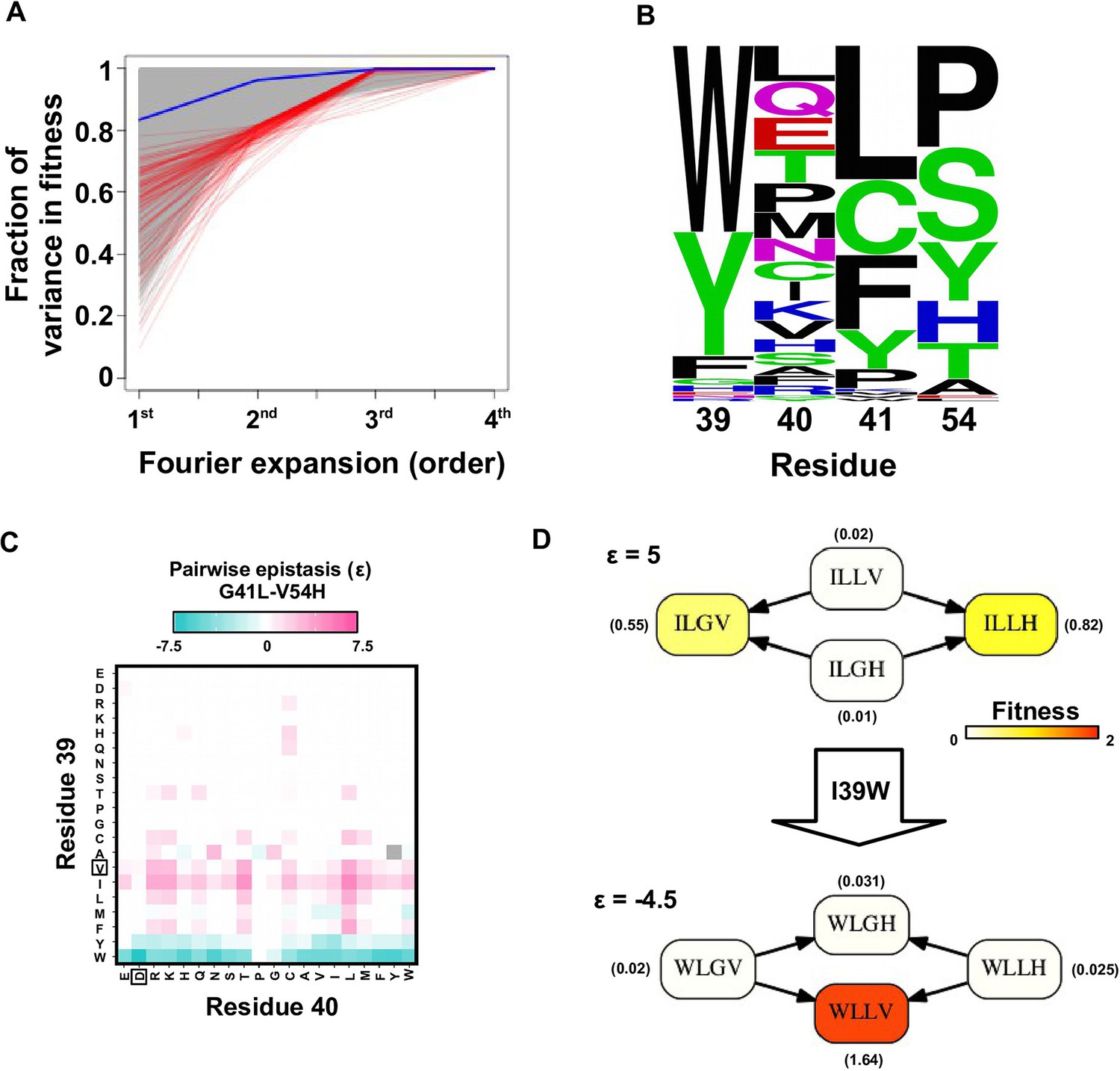
Evidence of higher-order epistasis.
(A) The fitness decomposition was performed on all subgraphs without missing variants. The fitness of variants can be reconstructed using Fourier coefficients truncated to a certain order. The fraction of variance in fitness explained by expansion of Fourier coefficients truncated to different orders (from first to fourth) is shown for each subgraph. The blue line corresponds to the median. The top 0.1% subgraphs with fitness contributions from higher-order epistasis (the bottom 0.1% subgraphs ranked by fraction of variance explained at second order expansion) are shown in red lines. (B) A sequence logo was generated for the quadruple mutants corresponding to the top 0.1% subgraphs with higher-order epistasis. The skewed composition of amino acids indicates that higher-order interactions are enriched among specific amino acid combinations of site 39, 41 and 54. (C) The magnitude of pairwise epistasis between G41L and V54H across different genetic backgrounds (i.e. all combinations of amino acids at site 39 and 40) is shown as a heat map. The amino acids of WT are boxed. Epistasis that cannot be determined due to missing variant is colored in grey. (D) Altering the genetic background at site 39 changed the positive epistasis () between G41L and V54H to negative epistasis (). The fitness of each variant is indicated in the parentheses.
Figure 3—figure supplement 1
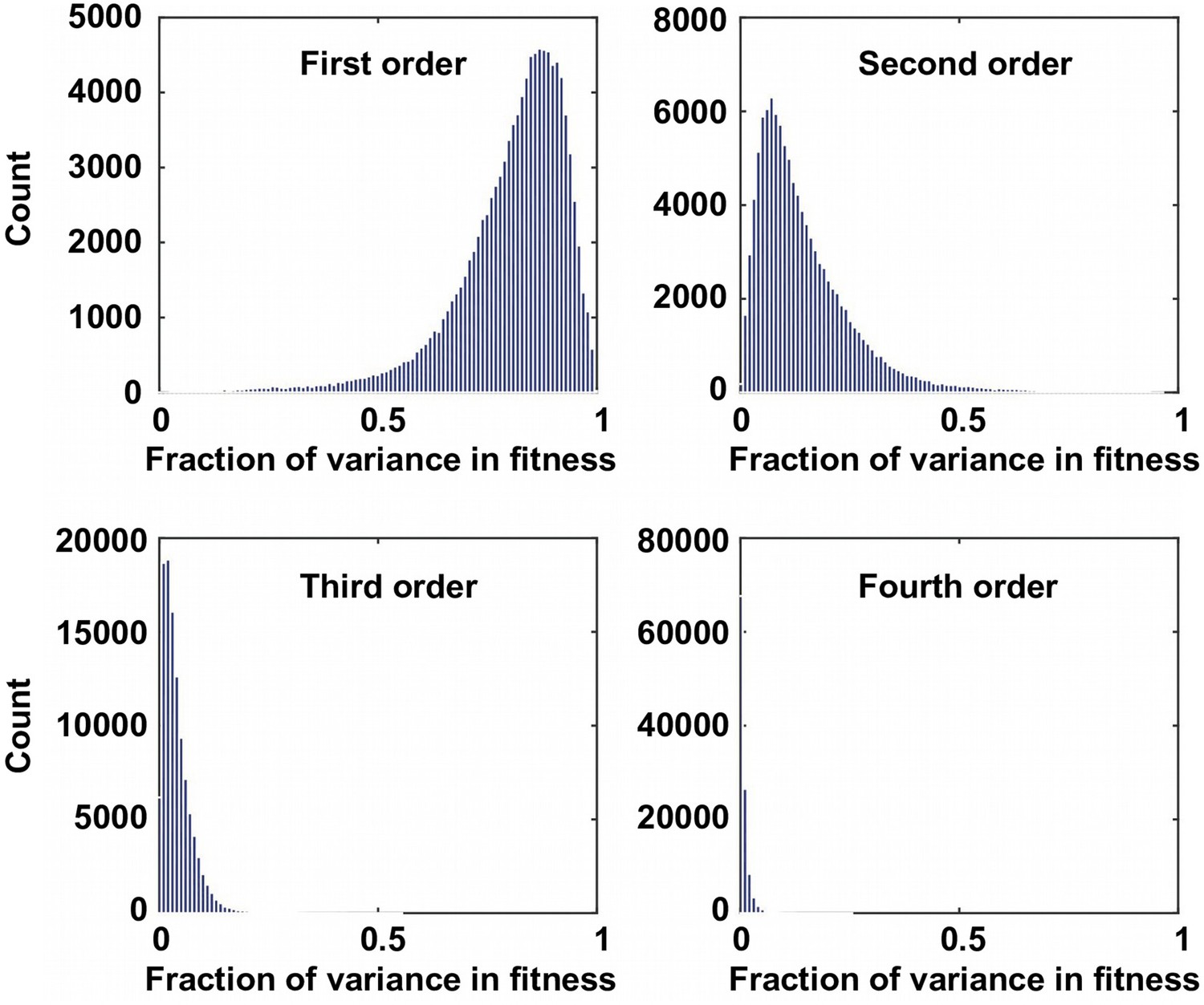
The fraction of variance explained by Fourier coefficients at each order.
For the 109,235 complete subgraphs that we analyzed, the fraction of the variance in fitness explained by each order is shown. Although the first order (main effects) and the second order Fourier coefficients (pairwise epistasis) can explain most of the variance in fitness, higher-order epistasis is present in certain combination of mutations.
Figure 3—figure supplement 2
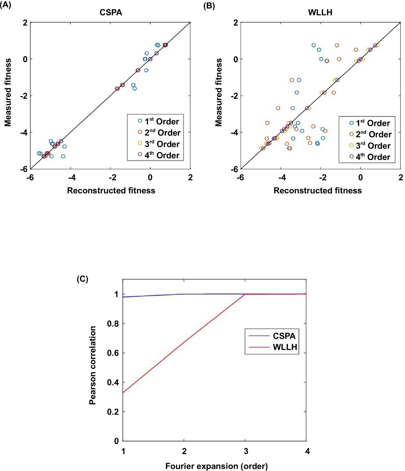
Fourier analysis decomposes the fitness landscape into epistatic interactions of different orders.
Here we show two examples where the fitness contribution from higher-order epistasis is small (bottom 0.1%, from VDGV to CSPA) in (A) and large (top 0.1%, from VDGV to WLLH) in (B). The fitness of variants can be reconstructed using Fourier coefficients truncated to a certain order. The Fourier coefficients can be interpreted as epistatic interactions of different orders, including the main effects of single mutations (the first order), pairwise epistasis (the second order), and higher-order epistasis (the third and the fourth order). (C) In our system with four sites, the reconstructed fitness by expansion to the fourth order Fourier coefficients will always reproduce the measured fitness (i.e. Pearson correlation equals 1). If expansion to the second order Fourier coefficients did not reproduce the measured fitness (i.e. Pearson correlation less than 1), it would indicate the presence of higher-order epistasis.
Figure 3—figure supplement 3
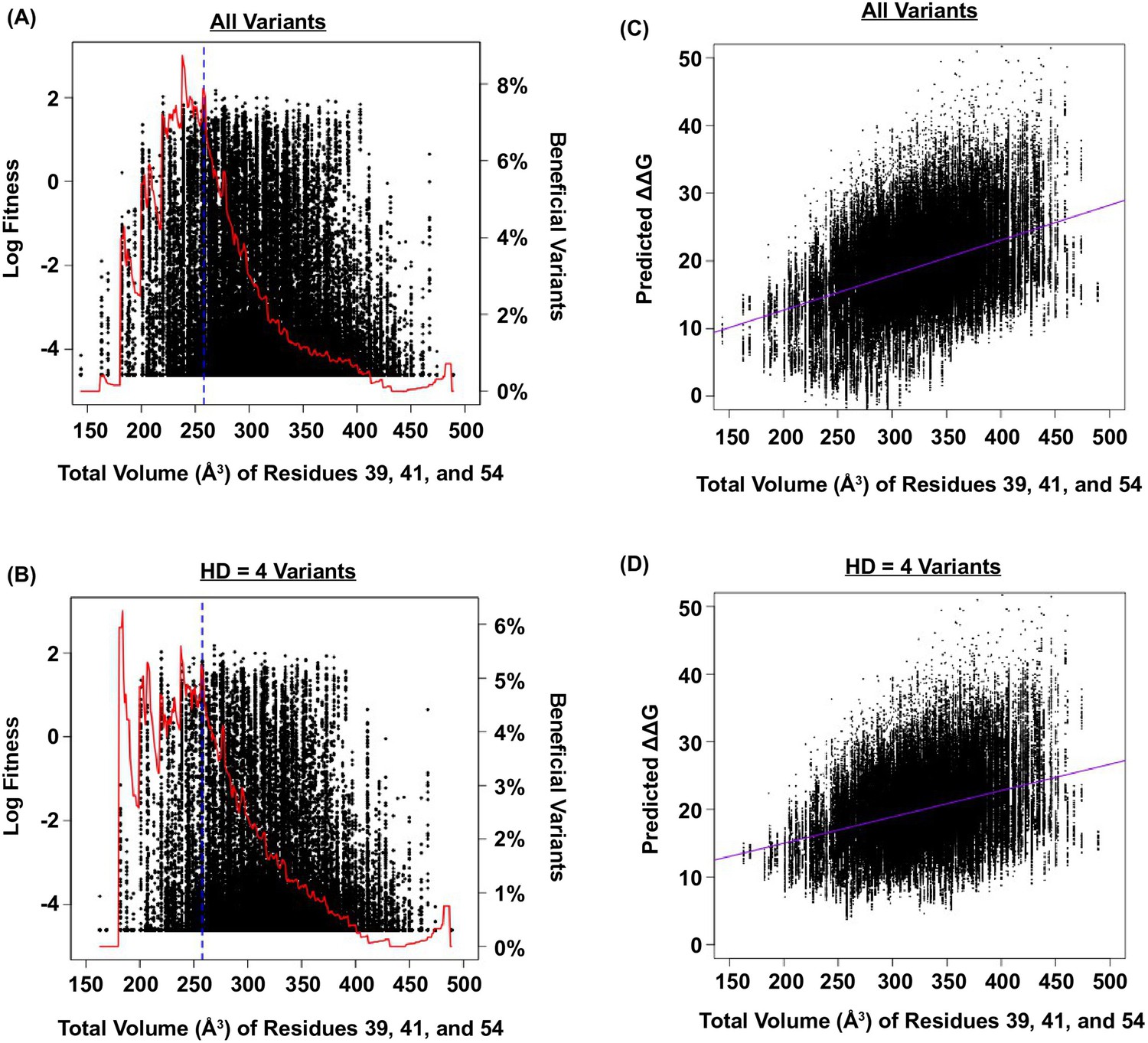
Relationship between fitness, size of the protein core, and predicted ΔΔG.
(A and B) The relationship between fitness and the total volume of residue 39, 41, and 54 is shown as a scatter plot for (A) all variants, and (B) variants with HD of 4 from WT. The blue line indicates the volume of WT (VDGV). The red line indicates the fraction of beneficial variants within a sliding window of 20 Å3. We postulated that the observed higher-order epistasis was, at least partially, due to the steric effect among site 39, 41, and 54. This was evidenced by the enrichment of beneficial variants when the total volume of these three interacting residues was between ~200 Å3 and ~300 Å3. As the total volume further increased, proportion of beneficial variants dropped. (C and D) The relationship between the predicted G and the total size of residue 39, 41, and 54 for all variants is shown as a scatter plot for (C) all variants (Pearson correlation = 0.41), and (D) variants with HD of 4 from WT (Pearson correlation = 0.34). The purple line represents the linear regression. The predicted G increased as the total volume of core residues increased, indicating that the protein would be destabilized (i.e. decrease in fitness) when the core was overpacked. Therefore, the higher-order epistasis observed in this study could be partially attributed to steric effect. Nonetheless, we acknowledged that entropic effect and conformational effect in IgG-FC binding may also contribute to higher-order epistasis.
Figure 3—figure supplement 4
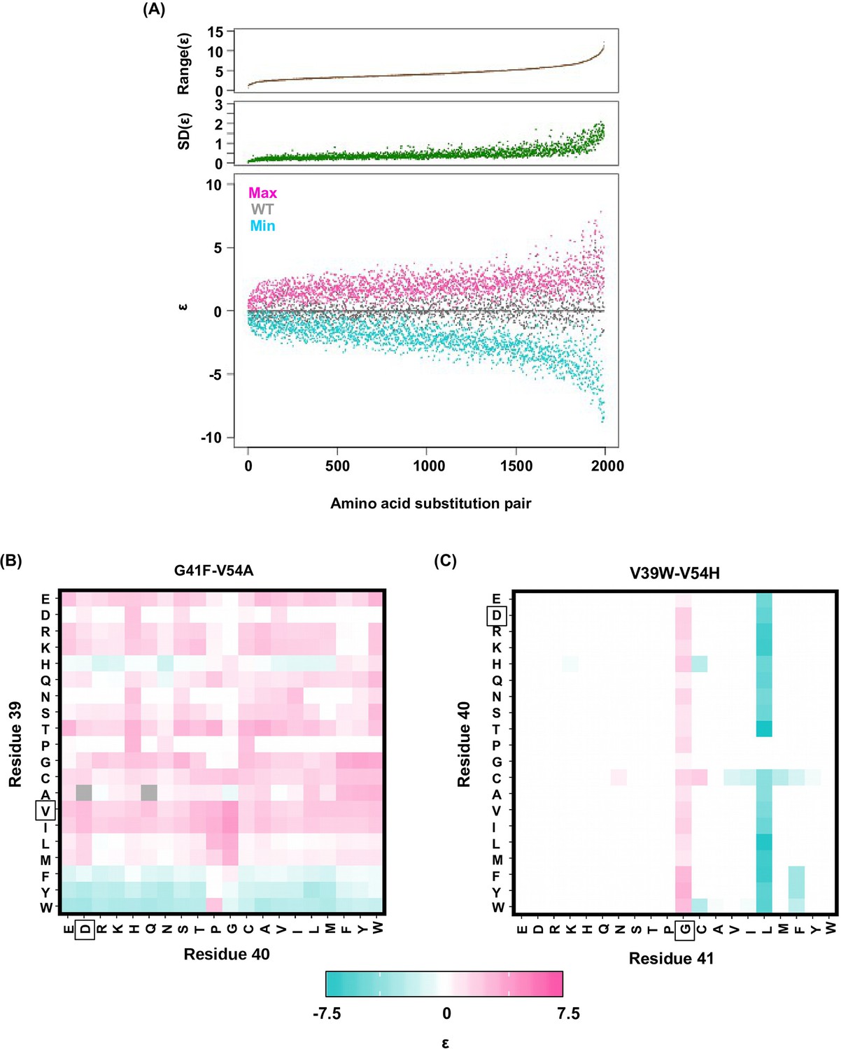
Alteration of pairwise epistatic effect under different genetic backgrounds.
(A) Pairwise epistatic effect of each substitution pair under each genetic background (total possible genetic backgrounds for each substitution pair = 20 × 20 = 400) was quantified. For each substitution pair, the range of epistasis across different genetic backgrounds is shown in the top panel (brown). For each substitution pair, the standard deviation of epistasis across different genetic backgrounds is shown in the middle panel (green). For each substitution pair, the maximum epistatic value across different genetic backgrounds (magenta), the minimum epistatic value across different genetic backgrounds (cyan), and the epistatic value under WT background (grey) are shown. Substitution pair is ranked by the range of epistasis (maximum epistatic value minus minimum epistatic value). (B) Epistasis between G41F and V54A across different genetic backgrounds (different combination of amino acids in sites 39 and 40) is shown. The epistasis value is color coded. Amino acids of WT are boxed. Epistasis that cannot be determined due to missing variant is colored in grey. (C) Epistasis between V39W and V54H across different genetic backgrounds (different combination of amino acids in sites 40 and 41) is shown. The epistasis value is color coded. Amino acids of WT are boxed. Epistasis that cannot be determined due to missing variant is colored in grey.
Figure 3—figure supplement 5
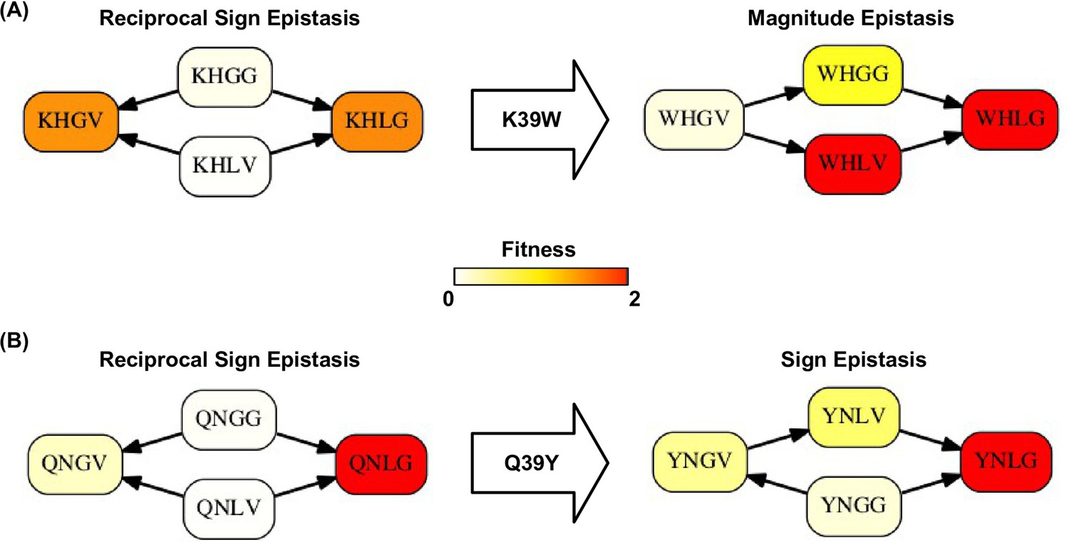
Higher-order epistasis can change the type of pairwise epistasis.
The type of pairwise interaction could be changed in the presence of higher-order epistasis. (A) Reciprocal sign epistasis between G41L-V54G is changed to magnitude epistasis given the mutation at site 39 (K39W). (B) Reciprocal sign epistasis between G41L-V54G is changed to sign epistasis given the mutation at site 39 (Q39Y).
Figure 3—figure supplement 6
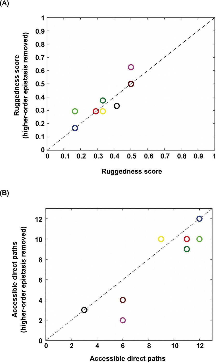
Higher-order epistasis increases the ruggedness of fitness landscapes.
To further study the effect of higher-order epistasis on landscape ruggedness, we performed additional analyses on the subgraphs identified in Figure 1B. We applied Fourier decomposition and set all higher-order coefficients to 0. (A) Among the subgraphs in which the quadruple mutant was still the only fitness peak, we found that the ruggedness score did not show a systematic trend after removal of higher-order epistasis. (B) In the meantime, on average the number of accessible direct paths seemed to decrease. Each data point is color-coded so that individual subgraphs can be matched between panel A and B.
Figure 4 with 4 supplements
Indirect paths promote evolutionary accessibility.
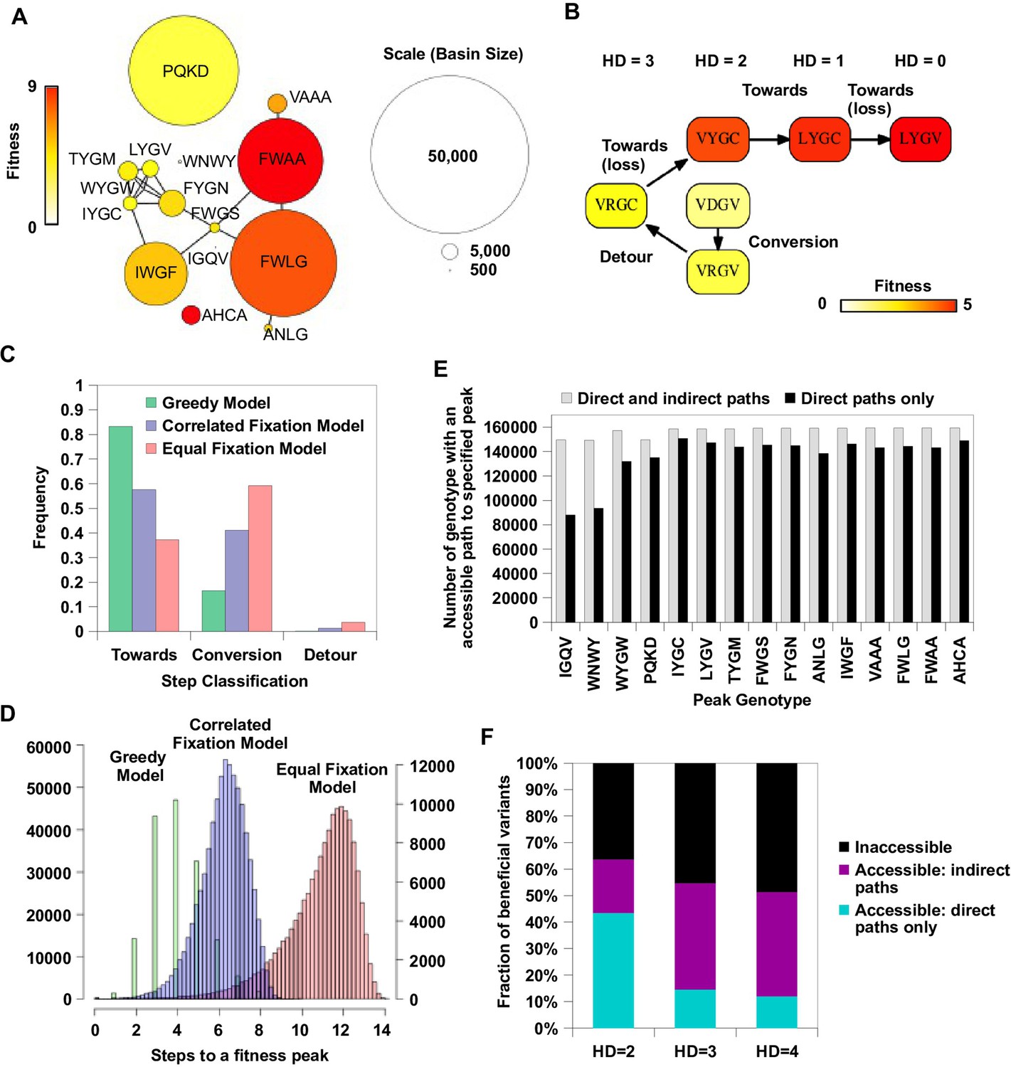
(A) 15 peaks had fitness larger than WT and their combined basins of attraction accounted for 99% of the entire sequence space. The size of each basin of attraction is identified by the Greedy Model (see Materials and methods). The area of each node is in proportion to the size of the basin of attraction of the corresponding fitness peak. An edge is drawn between fitness peaks that are separated by a Hamming distance of 2. (B) A possible adaptive path starting from WT (VDGV) to the fitness peak LYGV. (C) The frequency of different types of mutational step are shown. Three models, including the Greedy Model (green), Correlated Fixation Model (blue) and Equal Fixation Model (red), are used to simulate 1000 adaptive paths starting from each variant in the sequence space. All the adaptive paths end at a fitness peak. (D) The distribution of the length of the adaptive path initiated at different starting points. For Correlated Fixation Model and Equal Fixation Model, the length was computed by averaging over 1000 simulated paths for each starting point. The scale on the left is for Greedy Model. The scale on the right is for Correlated Fixation Model and Equal Fixation Model. (E) Indirect paths increased the number of genotypes accessible to each fitness peak. The 15 peaks are ordered by increasing fitness (from left to right). (F) A large fraction of beneficial variants in the sequence space (fitness > 1) were accessible from WT only via indirect paths. Beneficial variants were classified by their Hamming distance (HD) from WT.
Figure 4—figure supplement 1
Lasso regression.
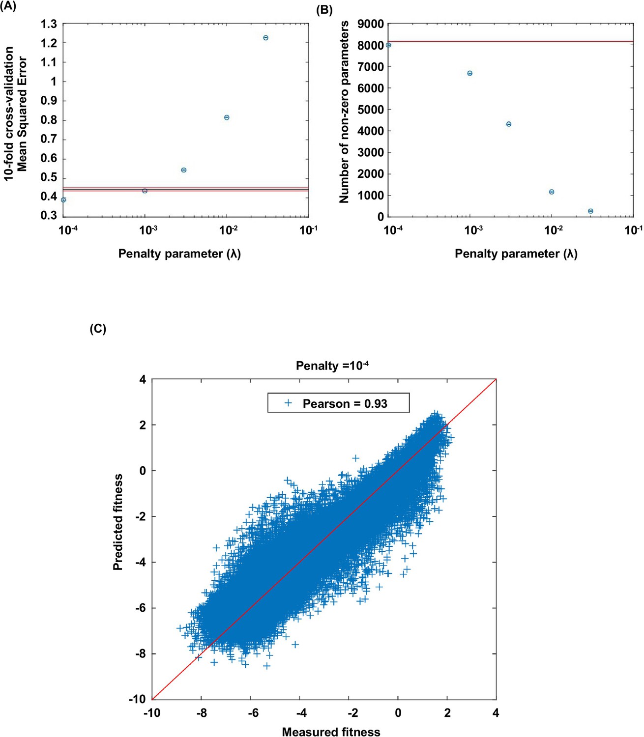
Coefficients of the statistical model were fit by lasso regression on the measured fitness values of 119,884 non-lethal variants (see Materials and methods). (A) 10-fold CV (cross-validation) MSE (mean squared errors) of lasso regression with varying penalty parameter . The black line indicates the 10-fold CV MSE of ordinary least squares regression (i.e. penalty parameter is zero). The red lines indicate the standard deviation. is chosen for imputing the fitness values of missing variants. (B) The number of nonzero coefficients in the model with varying penalty parameter . The line indicates the number of nonzero coefficients given by ordinary least squares regression. (C) Comparison between the predicted fitness values and the measured fitness values (Pearson correlation=0.93).
Figure 4—figure supplement 2
Indirect paths in adaptation.
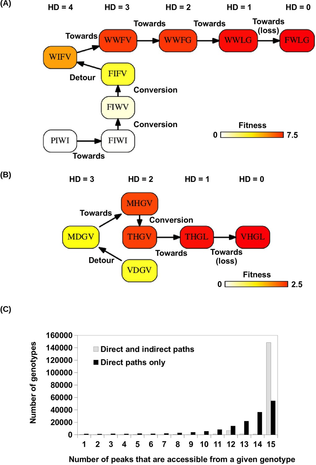
(A) A mutational trajectory initiated from PIWI under Greedy Model, which ended at the fitness peak, FWLG. (B) One of the shortest mutational trajectories from WT (VDGV) to a beneficial mutation (VHGL). (C) Histogram of the number of fitness accessible from a given genotype. The fraction of genotypes accessible to 15 fitness peaks increased substantially when indirect paths are allowed in adaptation.
Figure 4—figure supplement 3
Evolutionary accessibility under constraints imposed by the standard genetic code.
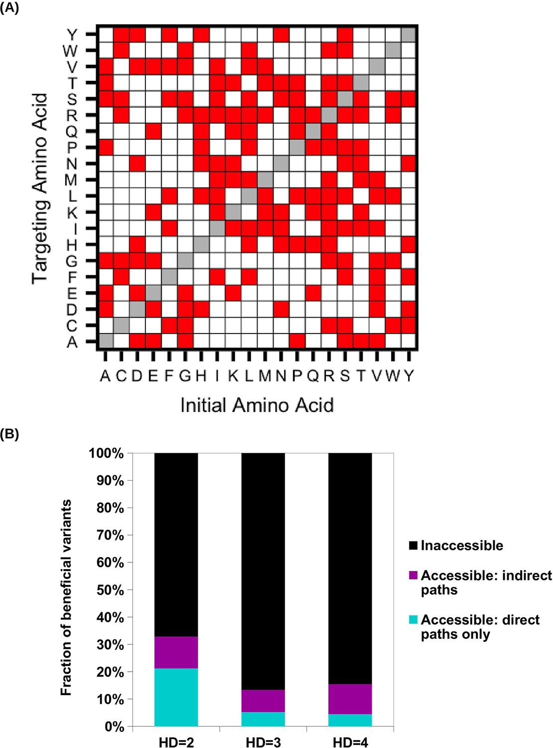
(A) To study evolutionary accessibility under constraints imposed by the standard genetic code, we restricted amino acid substitutions to those that were differed by a single nucleotide. This constraint is shown as a symmetric matrix, where red represents substitution that is allowed and white represents substitution that is not allowed. (B) Beneficial variants (fitness > 1) were classified by their Hamming distance (HD) from WT at the amino acid level. Accessibility to these beneficial variants from WT was determined under the constraints imposed by the standard genetic code.
Figure 4—figure supplement 4
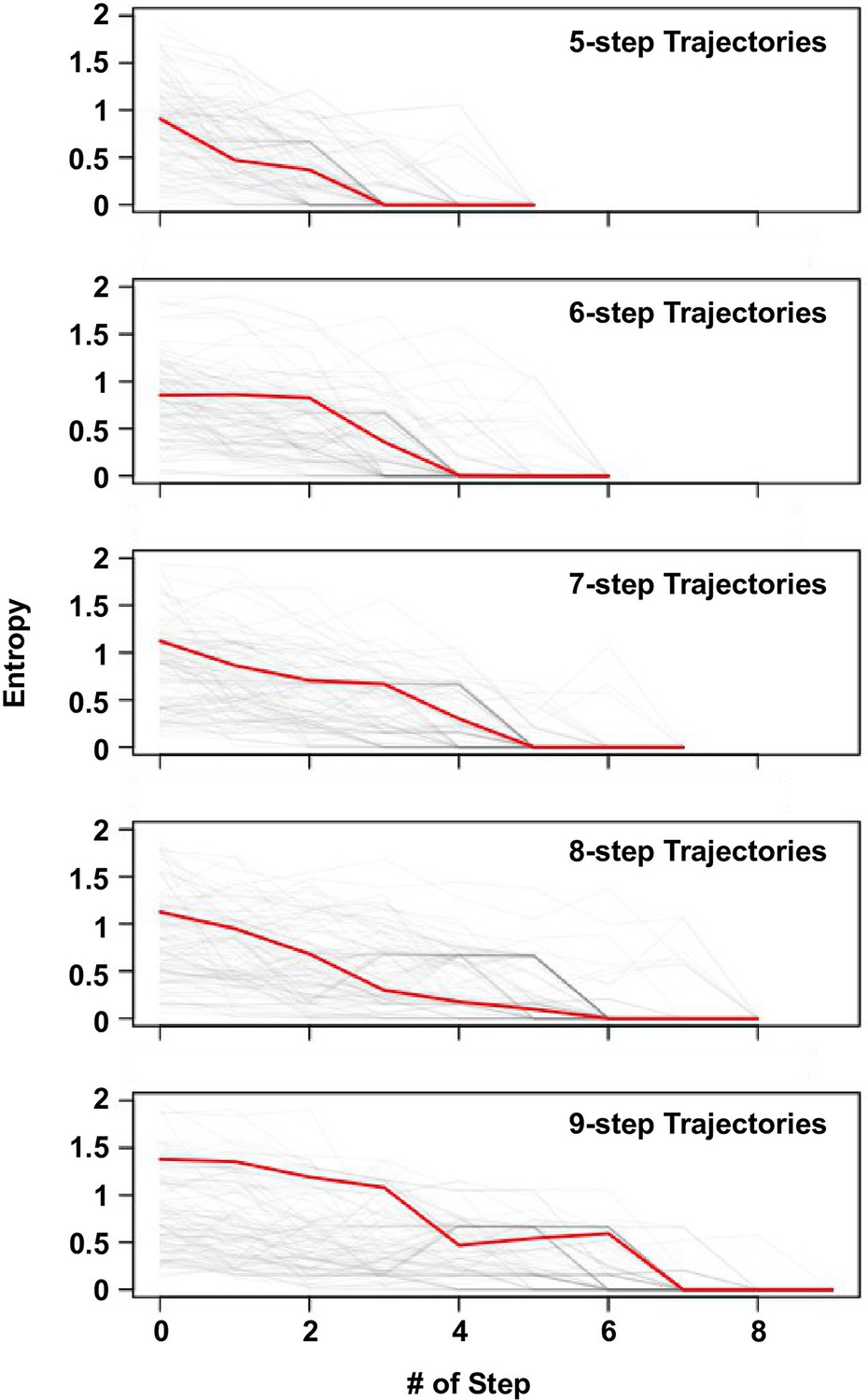
Delay of commitment in mutational trajectories involving extra-dimensional bypass.
An entropy of evolutionary outcome was calculated for each of the 160,000 variants. Given a variant with accessible fitness peaks, the entropy of evolutionary outcome was then computed as follow:
where represented the frequency of reaching the fitness peak among 1000 simulated mutational trajectories from variant following Correlated Fixation Model.
The entropy of evolutionary fates at each step along an adaptive path is shown. Adaptive paths with the same number of steps are grouped together. We observed that many mutational trajectories that involved extra-dimensional bypass did not fully commit to a fitness peak (entropy = 0) until the last two steps. Each grey line represents a mutational trajectory in each category. Only 100 randomly sampled trajectories are shown due to the difficulty in visualizing a large number of lines on the graph. The median entropy at each step in each category is represented by the red line.
Additional files
-
Supplementary file 1
The fitness of each profiled variant.
- https://doi.org/10.7554/eLife.16965.024
-
Supplementary file 2
Imputed fitness values for missing variants.
- https://doi.org/10.7554/eLife.16965.025
Download links
A two-part list of links to download the article, or parts of the article, in various formats.
Downloads (link to download the article as PDF)
Open citations (links to open the citations from this article in various online reference manager services)
Cite this article (links to download the citations from this article in formats compatible with various reference manager tools)
Adaptation in protein fitness landscapes is facilitated by indirect paths
eLife 5:e16965.
https://doi.org/10.7554/eLife.16965


