A map of abstract relational knowledge in the human hippocampal–entorhinal cortex
- Wellcome Trust Centre for Neuroimaging, Institute of Neurology, University College London, United Kingdom
- University of Oxford, United Kingdom
- Max Planck-UCL Centre for Computational Psychiatry and Ageing Research, United Kingdom
Figures
Figure 1 with 1 supplement

Experimental design.
(A) Graph structure used to generate stimulus sequences on day 1. Trial transitions were drawn from random walks along the graph. (B) Objects on reduced graph presented to subjects in the scanner on day 2. Trial transitions were random. In both sessions, participants performed simple behavioural cover tasks. See Figure 1—figure supplement 1 for behavioural performance during the training and the scan sessions. fMRI: functional magnetic resonance imaging.
Figure 1—figure supplement 1
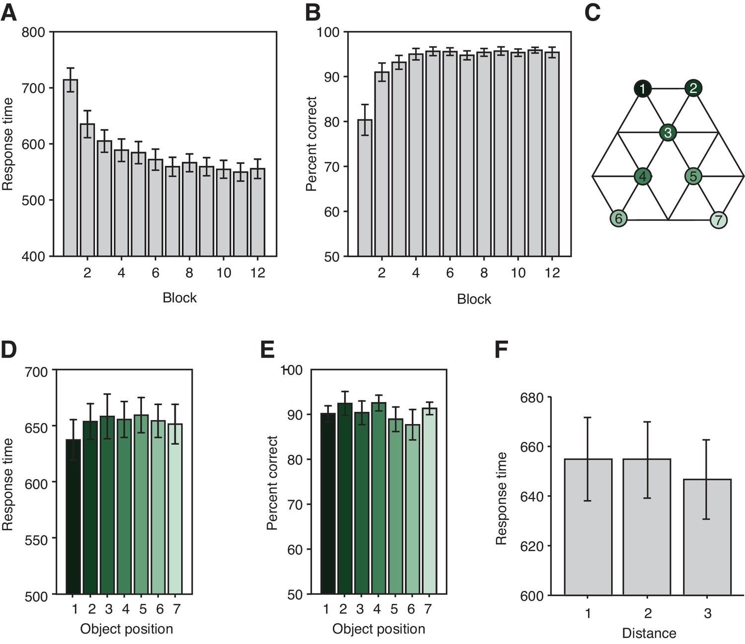
Task performance.
(A) Response times (ms) and (B) performance on the orientation judgment cover task performed during training on day 1 for each of the 12 blocks. (C) Graph structure indicating the object position. (D) Response times (F6,132 = 0.68, p=0.67) and (E) percent correct (F6,132 = 0.56, p=0.77) on the patch detection cover task performed during the functional magnetic resonance imaging experiment do not differ for the different object locations. (F) Response times on the patch detection cover task do not depend on the distance between objects on the graph (F2,44 = 0.72, p=0.49). Error bars show mean and standard error of the mean.
Figure 2 with 3 supplements
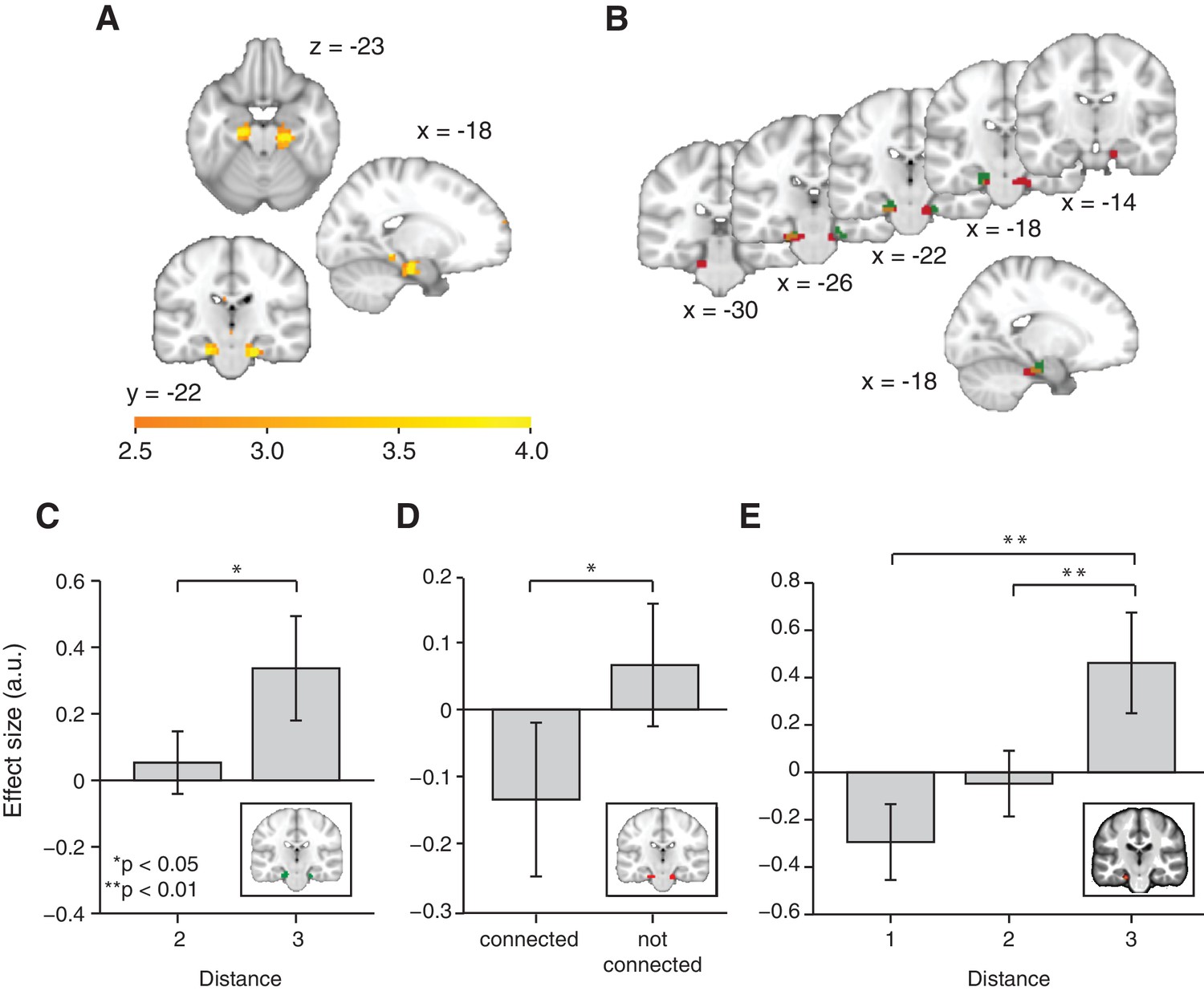
Functional magnetic resonance imaging adaptation in the hippocampal–entorhinal system decreases with distance on the graph.
(A) Whole-brain analysis showing a decrease in functional magnetic resonance imaging adaptation with link distance in the hippocampal–entorhinal system, thresholded at p<0.01, uncorrected for visualisation. (B) Within the hippocampal–entorhinal system, green indicates greater suppression if the preceding stimulus was a neighbour relative to a stimulus two or three links away. Red indicates greater suppression if a preceding stimulus was two links away than three links away. The depicted areas were used as regions of interest for analyses in (C) (green) and (D) (red). (C) Parameter estimates for link 2 versus link 3 transitions extracted from the green entorhinal region of interest in Figure 2B (t22 = 2.27, p=0.03). Other brain areas do not show this increase in activity with distance (Figure 2—figure supplements 2D,E). (D) Parameter estimates extracted from the red entorhinal region of interest in Figure 2B, sorted according to whether objects were connected on the graph or not (t22 = 2.34, p=0.03). (E) Parameter estimates extracted from the peak MNI coordinate reported in Chadwick et al. (2015), [−20, –25, −24] and sorted according to distance (F2,44 = 10.04, p=0.0003). See Figure 2—figure supplement 1 for masks used for small-volume correction in Figure 2A, Figure 2—figure supplement 2 for distance-dependent scaling effects in other brain regions and Figure 2—figure supplement 3 for effects of object familiarity and centrality. Error bars show mean and standard error of the mean. a.u.: arbitrary units.
Figure 2—figure supplement 1
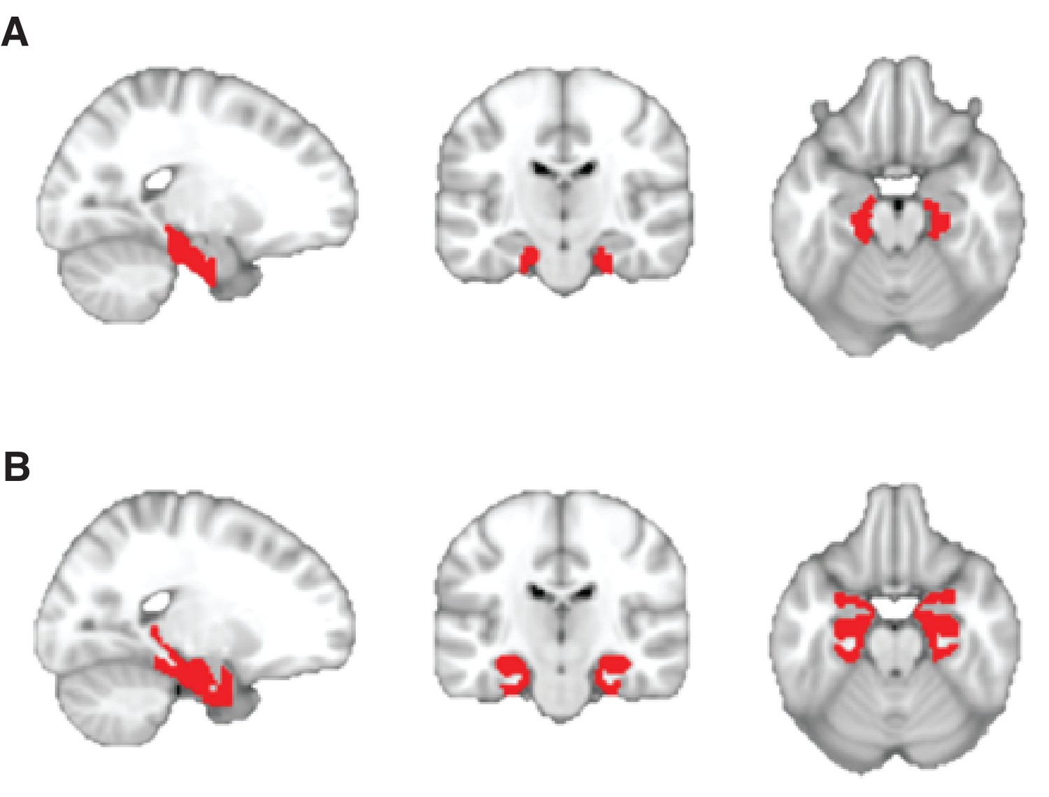
Anatomically defined regions of interest used for small-volume correction.
(A) Mask comprising the bilateral entorhinal cortex and subiculum, received with thanks from Chadwick et al. (2015). (B) Mask comprising the bilateral entorhinal cortex, hippocampus, and parahippocampal cortex. Regions were defined using the maximum probability tissue labels provided by Neuromorphometrics, Inc. (http://Neuromorphometrics.com).
Figure 2—figure supplement 2
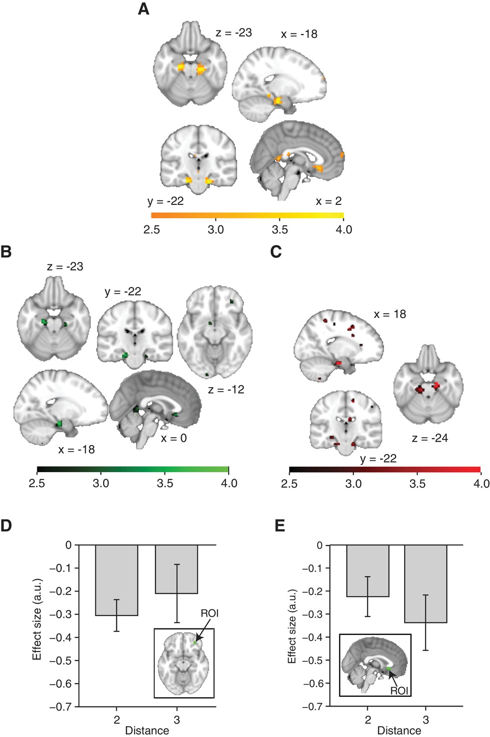
Distance-dependent scaling of neural activity is specific to the hippocampal–entorhinal system.
(A) All areas displaying a decrease in functional magnetic resonance imaging adaptation with graph distance. A cluster in the subgenual cortex did not survive whole-brain correction for multiple comparisons (punc=0.0008, pFWE=0.99, peak t22 = 3.58 [3, 23, −10]). (B) All areas displaying suppression for connected stimuli relative to non-connected stimuli on the graph. In addition to the hippocampal–entorhinal clusters reported in the main text, clusters in the orbitofrontal cortex (peak t22 = 2.93, [30, 41, −10]) and subgenual cortex (peak t22 = 3.33, [0, 23, −7]) were used to define regions of interest in order to test distance-dependent scaling, see (D, E). (C) All areas displaying greater suppression if a preceding stimulus was two links away rather than three links away. The corollary test for a difference in activity for connected versus non-connected objects was only significant in the hippocampal–entorhinal region of interest, see Figure 2B, D. (D) Parameter estimates for link 2 versus link 3 transitions extracted from the orbitofrontal cortex region of interest in (B). The difference is not significant (t22 = 0.85, p=0.41). (E) Parameter estimates for link 2 versus link 3 transitions extracted from the subgenual cortex region of interest in (B). The difference is not significant (t22 = 1.29, p=0.21). (A–C) are thresholded at p<0.01 for visualisation. Error bars show mean and standard error of the mean. a.u.: arbitrary units.
Figure 2—figure supplement 3
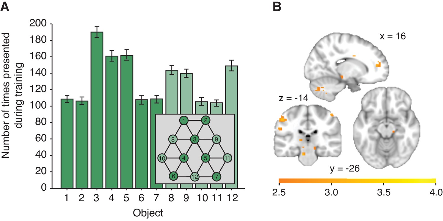
Effects of object familiarity.
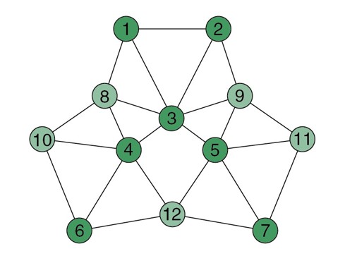
(A) Number of times each object was presented during training, averaged across participants. Note that this measure is directly related to the number of neighbours an object has on the graph. During scanning/behavioural testing, each object of the reduced graph depicted in dark green was presented equally often (180 times). Error bars denote standard deviation. (B) Decrease of activity with an increase in the number of times an object was presented during training (general linear model 3), thresholded at p<0.01 for visualisation. No cluster survives correction for multiple comparisons. No effect can be detected when testing for an increase of activity with an increase in the number of times an object was presented during training.
Figure 3 with 3 supplements
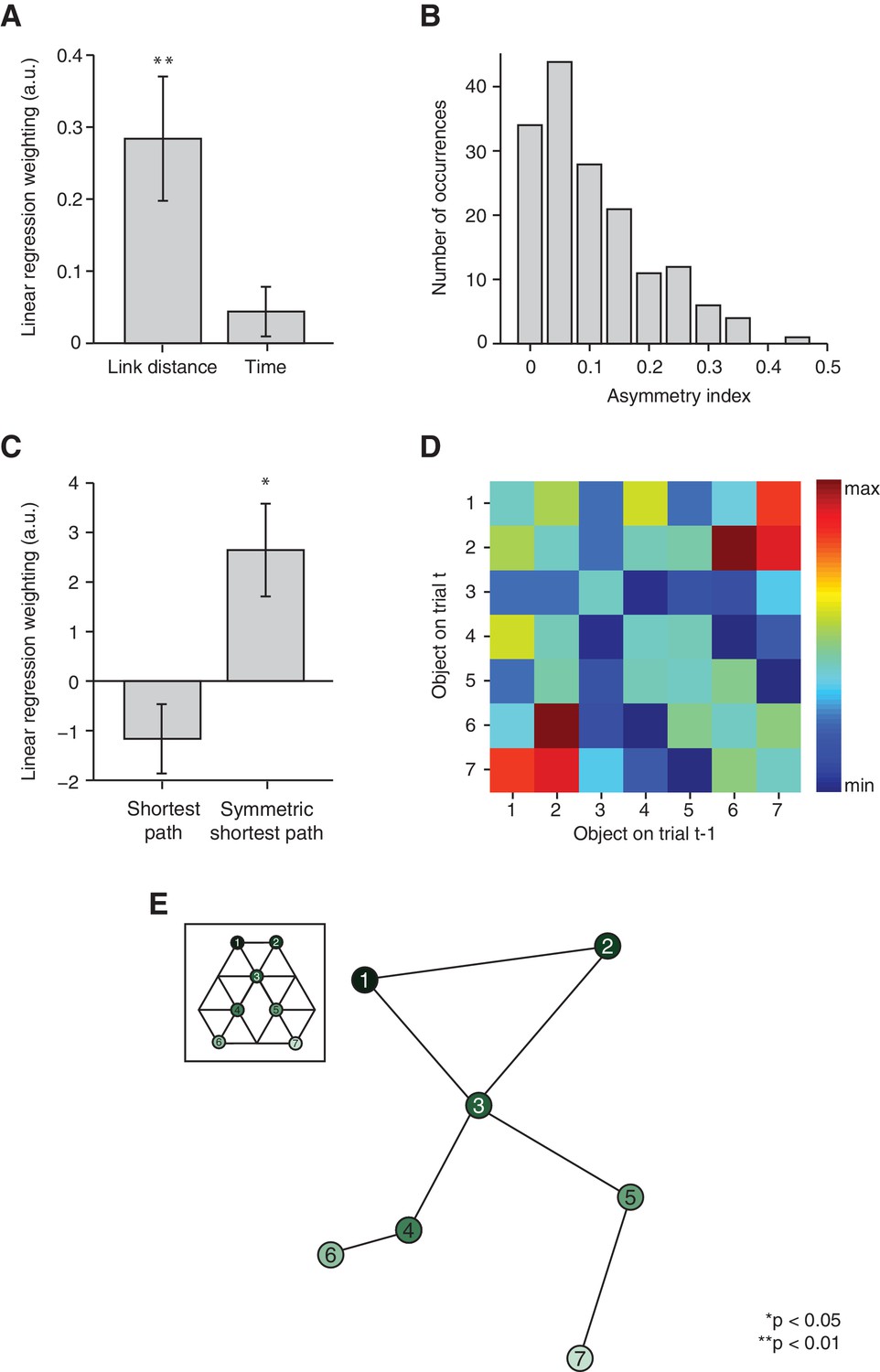
Relational information is organised as a map.
(A) Linear regression on neural activity with number of links and average time between two objects during training as regressors (t22 = 3.29, p=0.003 and t22 = 1.27, p=0.22). (B) Absolute difference in the number of times a transition was visited in one versus the other direction (e.g. 5 preceded by 1 vs. 1 preceded by 5) normalised by the total number of visits in either direction for all subjects. (C) Multiple linear regression on neural activity with the shortest path between objects and the symmetrised shortest path between objects as regressors (t22 = −1.64, p=0.11 and t22 = 2.78, p=0.01). (D) 7 × 7 matrix representing the average fMRI signal in response to an object depending on which other object preceded, averaged across subjects and symmetrised. Objects were never repeated during scanning; the diagonal entries are therefore set to 0. This matrix was used for the multidimensional scaling visualised in (E). (E) Visualisation of the localisation of the object representations in a two-dimensional space according to multidimensional scaling. Lines indicate transitions experienced during training. The distances between the resulting locations of nodes in a two-dimensional space are significantly correlated with the link distances of the original graph structure (r = 0.65, p=0.003, see Figure 3—figure supplement 2 for the null distribution used for the permutation test). All analyses were performed on data extracted from the peak MNI coordinate reported in Chadwick et al. [2015]), [−20, –25, −24], but also hold in an anatomically defined region of interest including the entorhinal cortex and the subiculum (Figure 3—figure supplement 3). See Figure 3—figure supplement 1 for results if object-specific activity is removed. Error bars show mean and standard error of the mean. a.u.: arbitrary units.
Figure 3—figure supplement 1

The distance-dependent scaling cannot be driven by a main effect of object position.
Position-specific activity in the region of interest (ROI) defined according to (A) a connected < non-connected contrast (ROI 1, Figure 2B, green, F6,132 = 0.88, p=0.5), (C) a link 2 < link 3 contrast (ROI 2, Figure 2B, red, F6,132 = 1.96, p=0.08) and (E) the peak coordinate in Chadwick et al. (2015) (ROI 3, F6,132 = 1.86, p=0.09). The tests reported in Figure 2C–E are also significant if performed after removing object-specific activity from the neural data. This was achieved by subtracting the mean activity for each object before testing for (B) a difference in activity for link 2 versus link 3 transitions in ROI 1 (t22 = 2.10, p=0.048), (D) a difference in activity for connected versus non-connected stimuli in ROI 2 (t22 = 2.39, p=0.03), or (F) a distance effect in ROI 3 (F2,44 = 6.68, p=0.003). Error bars show mean and standard error of the mean. a.u.: arbitrary units.
Figure 3—figure supplement 2
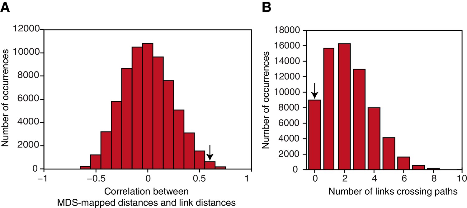
Map characteristics in a null distribution generated by permuting the links making up the graph structure.
(A) Correlation of link distances for graphs making up the null distribution with distances resulting from performing multidimensional scaling on the neural data. The null distribution was constructed by permuting the seven links making up the reduced graph structure to a random set of nodes. The correlation between link distances for the actual graph structure and distances resulting from MDS on the neural data is 0.65. Only 0.28% of graphs show a correlation with the mapped data of 0.65 or higher. (B) Number of line crossings for graphs characterised by nodes in the same location as given by the MDS procedure, but with the seven links randomly distributed between nodes. Only 13.17% of all possible graphs generated in this way are characterised by no line crossings; 0.25% of all graphs have no line crossing and a correlation of 0.65 or higher. The arrows indicate the corresponding measure for the actual data. MDS: multidimensional scaling.
Figure 3—figure supplement 3

Distance effects in an anatomically defined region of interest comprising the entorhinal cortex and the subiculum.
(A) Activity scales linearly with link distance (F2,44 = 8.41, p=0.0008). Post-hoc pairwise comparisons revealed a significant difference between distances of lengths 1 and 2 (t22 = 2.36, p=0.03), lengths 1 and 3 (t22 = 3.51, p=0.002), and lengths 2 and 3 (t22 = 2.23, p=0.04). (B) In a multiple linear regression, link distance, but not time, predicts the neural activity (t22 = 2.13, p=0.04 and t22 = 1.23, p=0.23). (C) In a multiple linear regression with symmetrised and non-symmetrised distance measures competing for variance, symmetrised distance rather than non-symmetrised distance explains the neural signal (directional distance: t22 = −1.27, p=0.22, symmetrised distance: t22 = 2.41, p=0.02). (D) The graph structure can be recovered by performing multidimensional scaling on the average functional magnetic resonance imaging data across subjects (r = 0.58, p=0.008, permutation test). Data for all analyses are extracted from the anatomically defined regions of interest shown in Figure 2—figure supplement 1A. Error bars show mean and standard error of the mean. a.u.: arbitrary units.
Figure 4 with 1 supplement
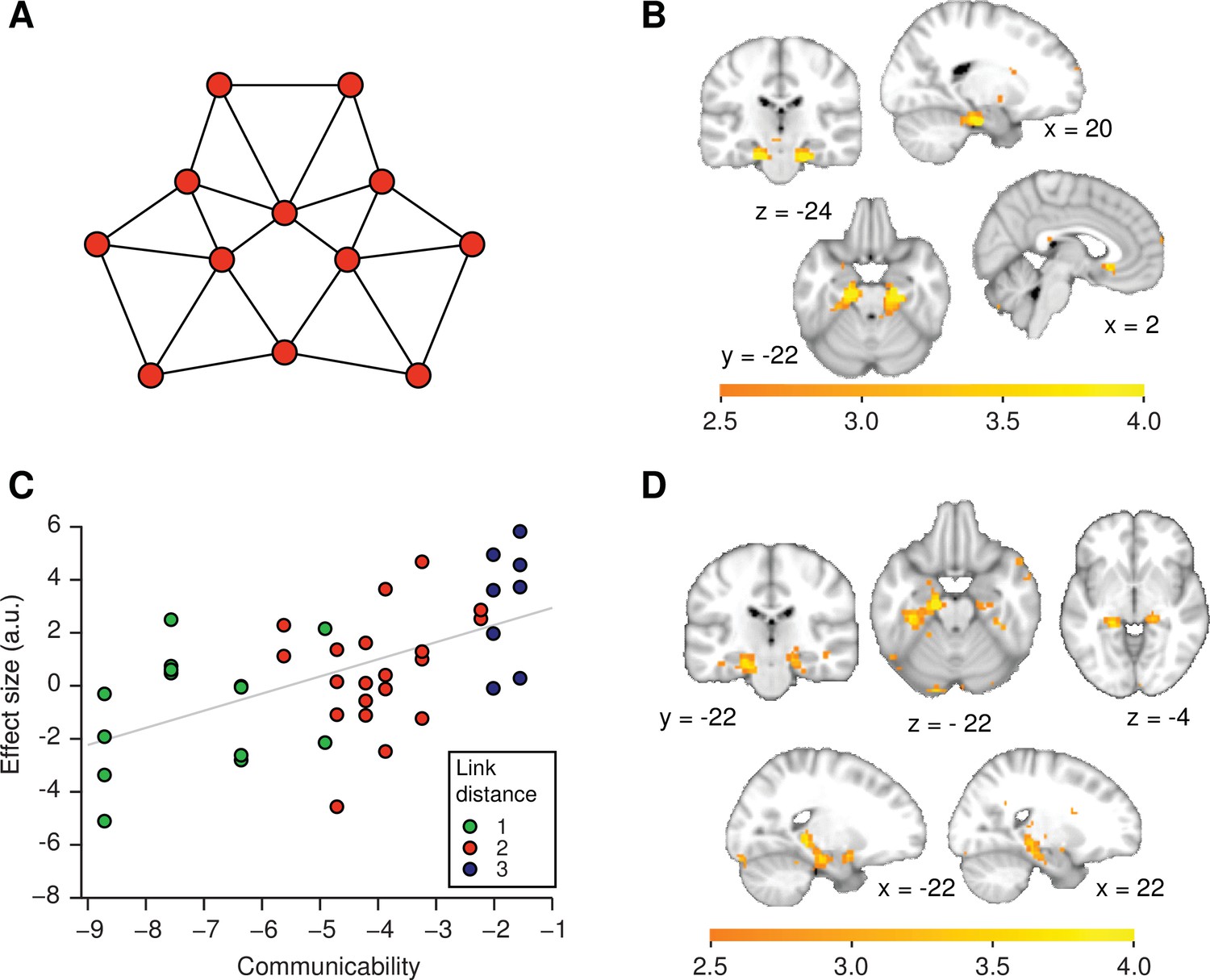
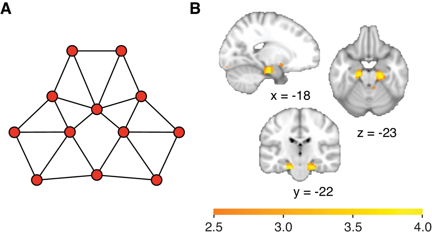
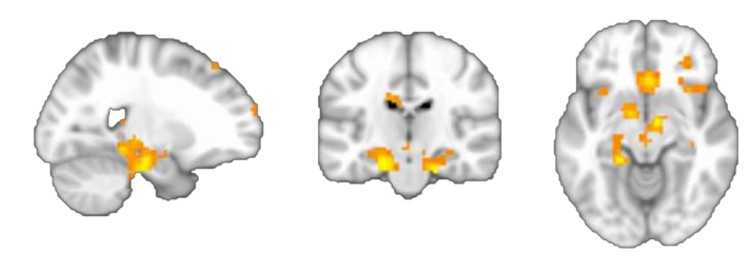
Functional magnetic resonance imaging adaptation in the hippocampal–entorhinal system is consistent with predictive representations of relational knowledge.
(A) Visualisation of communicability coordinates for the graph structure by performing multidimensional scaling on the communicability matrix. (B) Whole-brain regression of communicability onto neural activity. (C) Visualisation of the communicability effect. Average parameter estimate for each of the 42 stimulus transitions across subjects extracted from a bilateral region of interest in (B) (thresholded at p<0.01). The colours of the dots correspond to link distances. This graph is added for visualisation purposes only as the parameter selection is biased. (D) Whole-brain regression of communicability onto neural activity when Euclidian distances are included as an additional regressor in the general linear model. All statistical maps are thresholded at p<0.01 for visualisation. a.u.: arbitrary units.
Figure 4—figure supplement 1
Activity in the hippocampal–entorhinal system is consistent with the successor representation.
(A) Visualisation of successor representation coordinates for the graph structure by performing multidimensional scaling on the negative of the successor representation, with the free parameter set to ( = largest eigenvalue of the adjacency matrix ). (B) Whole-brain regression of the negative of the successor representation onto neural activity, with , reveals linear scaling with the successor representation in the hippocampal–entorhinal formation (family-wise error corrected at peak level within a bilateral entorhinal cortex/subiculum mask, left p=0.005, peak t22 = 4.80 [−18, –19, −25] and right p=0.007, peak t22 = 4.66, [24, −22, −25]. Both clusters also survived small volume correction for a larger region of interest comprising the hippocampus, parahippocampal cortex, and entorhinal cortex, left p=0.02 and right p=0.03, see regions of interest in Figure 2—figure supplement 1B). The statistical maps are thresholded at p<0.01 for visualisation.
Figure 5
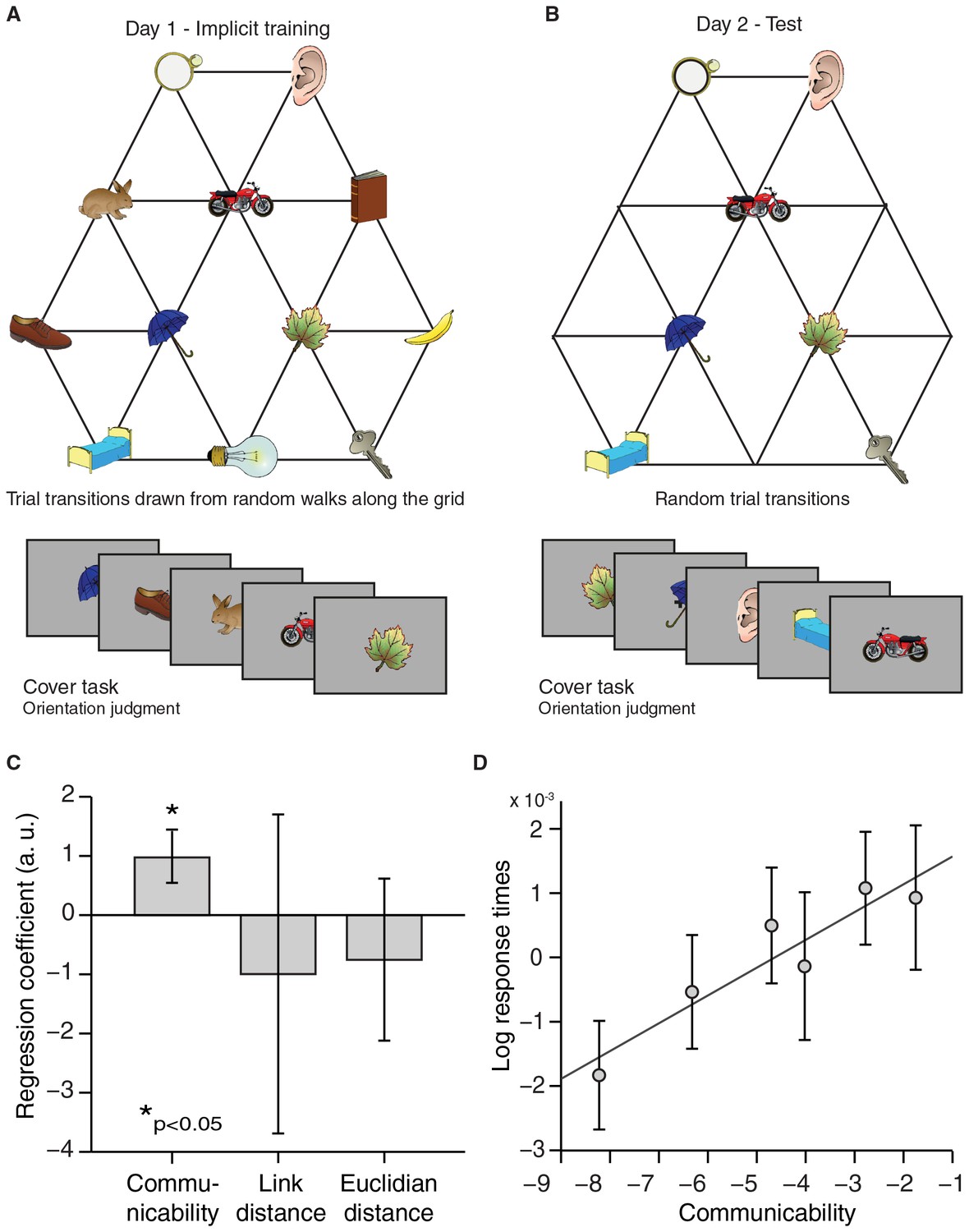
Response times reflect graph structure.
(A) Graph structure used to generate stimulus sequences on day 1. Trial transitions were drawn from random walks along the graph structure. (B) Objects on reduced graph presented to subjects on day 2. Trial transitions were random. In both sessions, participants performed an object orientation cover task under which response times were measured. (C) A regression of communicability, link distance, and Euclidian distance onto log-transformed response times across subjects (communicability: t25 = 2.77, p=0.01; link distance: t25 = −0.40, p=0.69; Euclidian distance: t25 = −0.85, p=0.40). (D) Visualisation of the relationship between communicability and log-transformed response times. Communicability measures were divided into six bins with an equal number of object–object transitions per bin. The y-axis corresponds to the average demeaned log-response time across subjects for each bin. Error bars denote the standard error of the mean. a.u.: arbitrary units.
Author response image 1
Visualisation of communicability coordinates for the graph structure by performing multi- dimensional scaling on the communicability matrix.
https://doi.org/10.7554/eLife.17086.016
Author response image 2
Download links
A two-part list of links to download the article, or parts of the article, in various formats.
Downloads (link to download the article as PDF)
Open citations (links to open the citations from this article in various online reference manager services)
Cite this article (links to download the citations from this article in formats compatible with various reference manager tools)
A map of abstract relational knowledge in the human hippocampal–entorhinal cortex
eLife 6:e17086.
https://doi.org/10.7554/eLife.17086


