The influence of evidence volatility on choice, reaction time and confidence in a perceptual decision
- Howard Hughes Medical Institute, Columbia University, United States
Figures
Figure 1
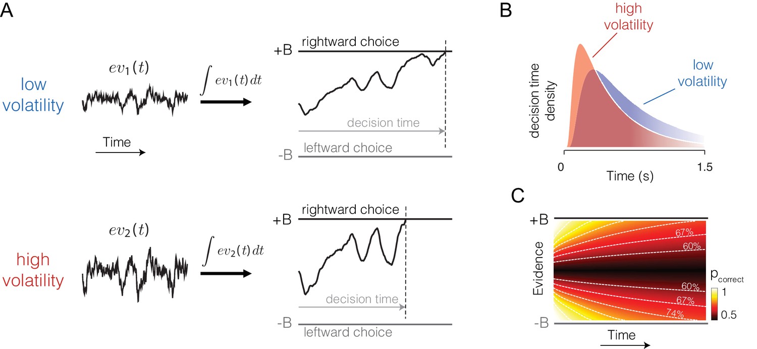
Predicted influence of volatility on reaction time and confidence under bounded evidence accumulation.
(A) ev1(t) and ev2(t) represent the time course of momentary evidence, for stimuli of low and high volatility, respectively. In bounded accumulation models, momentary evidence is integrated over time, until the accumulated evidence (decision variable, DV) crosses one of two bounds, here at ± B. Bound-crossing simultaneously resolves the choice that is made and the time it takes to make it (decision time; the reaction time also includes a nondecision component, not shown). With greater noise, the decision variable tends to diffuse more rapidly, leading to faster responses. (B) Illustration of the effect of volatility on the distribution of decision times, for two bounded accumulation models that have the same drifts and bound heights but different diffusion coefficients. As in the single trial example, higher variance leads to faster responses. (C) Heat map depicting the association between the state of accumulated evidence and the probability that a decision rendered on this evidence is correct. The structure in this graph arises because there are several difficulty levels. More reliable stimuli (e.g., high motion coherence), which support high accuracy, contribute to large vertical excursions of the decision variable away from the starting point (midpoint of the ordinate) at short elapsed time, whereas less reliable stimuli contribute to equivalent vertical excursions at later times. Example probability contours are depicted with dashed lines. Because the volatility of the stimulus is not explicitly represented in this map, higher volatility would lead to greater confidence, because the decision variable diffuses more quickly from the starting point, leading paradoxically to states that are normally associated with more reliable sources.
Figure 2 with 1 supplement
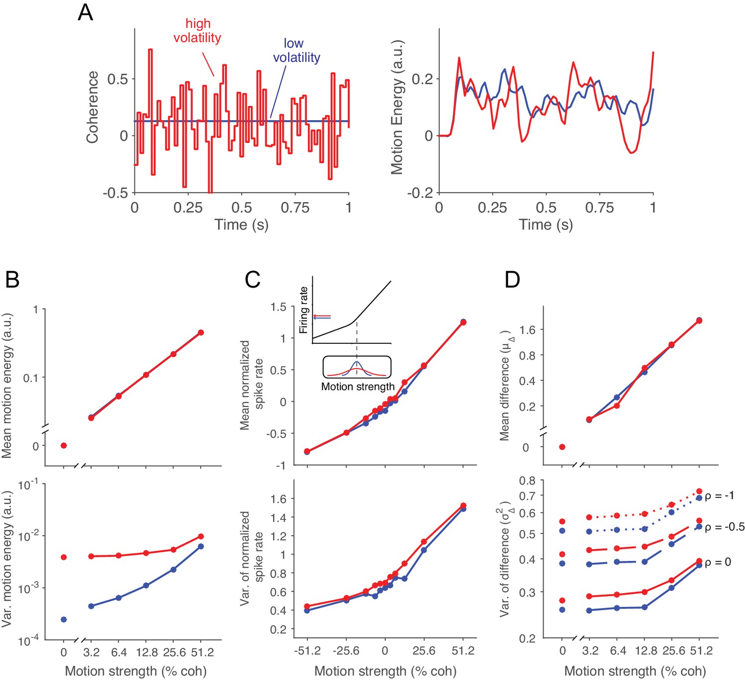
Doubly stochastic random dot motion selectively influences the variance of evidence.
Low and high volatility conditions are indicated by blue and red, respectively, in all panels. (A) Motion strength as a function of time for example stimuli with low and high volatility. Left: the coherence parameter is 0.128 for both stimuli, but in the high volatility condition this is the mean of a Gaussian distribution (S.D. = 0.256) that is sampled on every video frame (75 Hz). Right: motion energy in favor of the positive direction. Both volatility conditions yield variation in the motion information, but the red curve exhibits more variation. (B) Mean and variance of the motion energy in support of the true direction of motion, computed separately for trials of low and high volatility (N = 66,805 trials). For all motion strengths, the mean (upper) is not affected by the volatility manipulation, whereas the variance is larger in the high volatility condition. Note the log scale for both axes. (C) Mean and variance of the neuronal response from direction selective neurons in areas MT/MST (N = 26 single units and 21 multiunit sites; see Materials and methods). Spike counts were obtained from a 100 ms window beginning 100 ms after stimulus onset and standardized (z-score) for each neuron or multiunit site. The volatility manipulation produced a small increase in the average firing rate at the low coherences (upper). This increase is likely due to the rectification of the noise by the nonlinear response of the neuron to motion in the preferred and anti-preferred directions, as sketched in the inset. The variance parallels the mean, but volatility has a more marked effect on variance at weak motion strengths. Note the linear scales. (D) Mean and variance of a difference between opposing pools of neural signals. The graphs extrapolate from panel C by constructing two pools of 100 or more neurons sharing a common preferred or anti-preferred direction, respectively. The mean of the difference variable () is similar for both volatility conditions (upper), whereas the variance of the difference variable () is greater under high volatility (lower). This relationship is shown for three values of correlation () between the pools which span the plausible range. The correlation is negative because the opposing pools respond oppositely to fluctuations in the motion stimulus.
-
Figure 2—source data 1
Mean and variance of the neuronal response and of a difference variable between pools of neurons with opposite direction preferences.
- https://doi.org/10.7554/eLife.17688.005
Figure 2—figure supplement 1
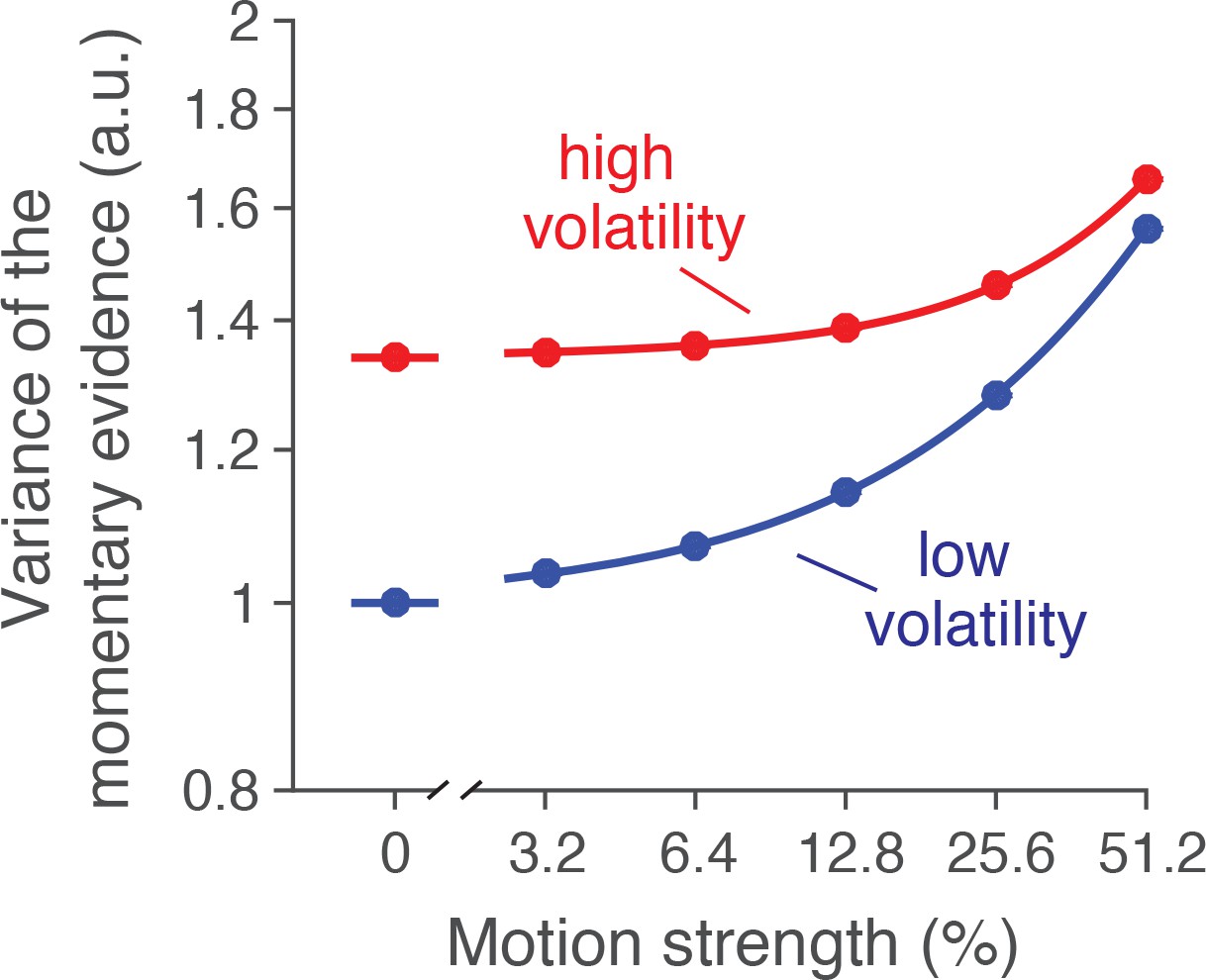
Variance of the momentary evidence from model fits.
In addition to the estimate of variance from neural recordings, we used a 3-parameter characterization of the noise as a function of volatility and motion strength. The example is from the fit to behavioral data from monkey W in the reaction-time task. See Materials and methods for details. Note the similarity of this graph to the estimates derived from the neural recordings in Figure 2D (lower panel).
Figure 3 with 1 supplement
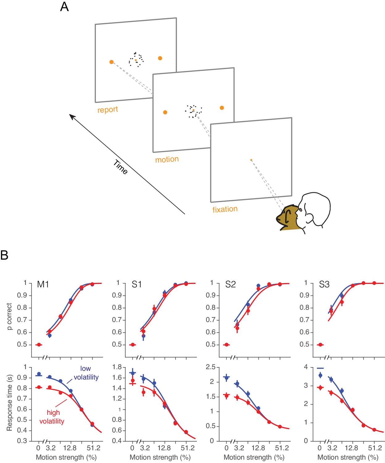
Effect of volatility on accuracy and reaction time.
(A) Choice-reaction time task. One monkey and three humans were required to make a decision about the net direction of motion in a dynamic random dot display. Subjects reported their decision by making a saccadic eye movement to the right (left) target for rightward (leftward) motion. They could report their decisions at any time after the onset of motion. Trials of different coherences and volatilities were randomly interleaved. (B) Decision speed and accuracy. Each column represents a different subject. High volatility had only weak effects on accuracy (upper) but shortened the reaction times for all subjects (lower), particularly at the low motion strengths. Symbols are mean ± s.e. Solid traces are fits of a bounded evidence accumulation (drift diffusion) model. (M1, monkey; S1-S3, human subjects).
-
Figure 3—source data 1
Accuracy and reaction times from the choice-reaction time task.
- https://doi.org/10.7554/eLife.17688.009
Figure 3—figure supplement 1

Accuracy in low and high volatility.
Although the volatility manipulation led to only a subtle reduction in overall accuracy, which was not statistically reliable, we believe this is because the volatility manipulation was attenuated at intermediate and strong motion strengths (Figure 2). Nevertheless, a small reduction in accuracy is apparent when examining only these intermediate and higher coherences. (A) For the data from the RT task, the scatter plot shows the average accuracy for low vs. high volatility. Each point represents a particular combination of subject and motion strength. The 0% and 51.2% coherences are not shown. Errors bars represent s.e. (B) Same as A, but including trials from all experiments (RT, PDW and human confidence tasks).
Figure 4 with 1 supplement
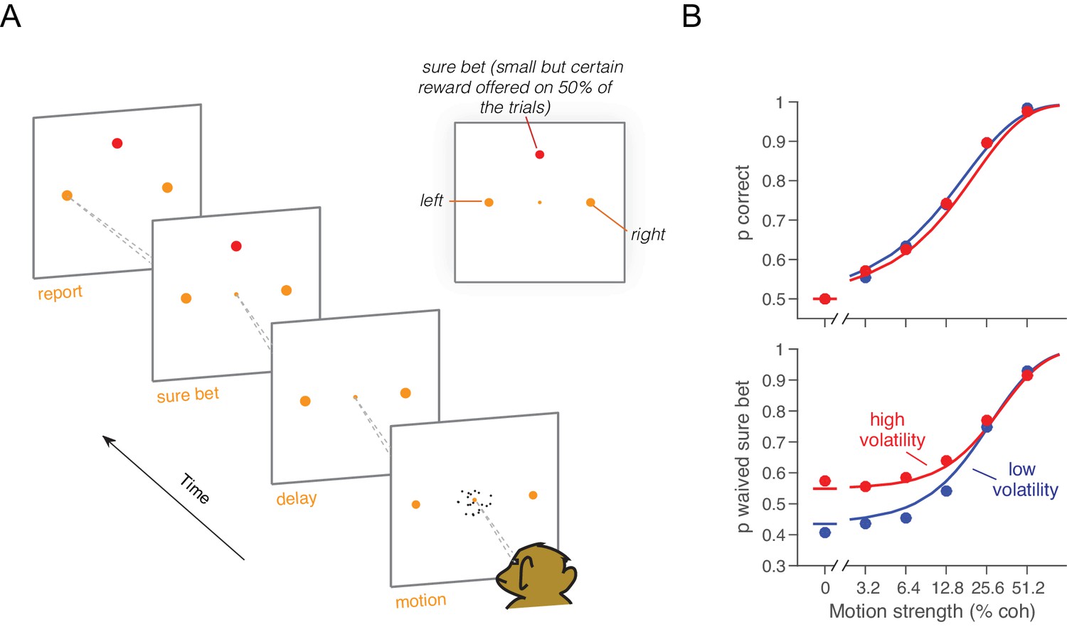
Effect of volatility on post-decision wagering.
(A) Task. The monkey viewed the motion display for random duration, controlled by the computer, followed by a memory-delay period. When the fixation point was extinguished, the monkey indicated the net direction of motion by making an eye movement to a left or right choice target in order to receive a liquid reward, if correct. On a random half of trials, the monkey was presented a third ‘sure bet’ option (red target) during the delay period, which if chosen resulted in a small but certain reward. (B) Decision confidence and accuracy. Volatility did not affect accuracy systematically (upper), but the monkey waived the sure bet option more often on trials employing the high volatility display (lower), indicating greater confidence. The effect was concentrated at weak and intermediate motion strengths. Standard errors are shown but are smaller than the symbols. Solid traces are model fits (see Materials and methods).
-
Figure 4—source data 1
Proportion of correct and waived direction choices as a function of motion strength and volatility condition in the PDW task.
- https://doi.org/10.7554/eLife.17688.012
Figure 4—figure supplement 1
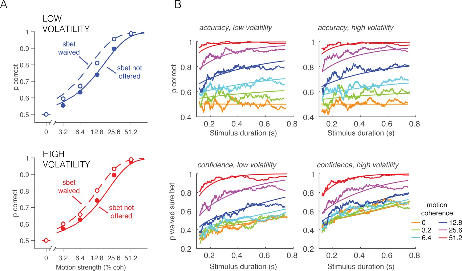
Accuracy and PDW behavior as a function of stimulus duration and sure-target availability.
(A) Accuracy in the direction discrimination task was better when the monkey waived the sure-bet target (open symbols) than when it was not offered (filled symbols). Solid and dashed curves are model fits. By opting out of the direction decision on trials in which the evidence seemed unreliable, the monkey improved its accuracy on trials in which it waived the sure bet option and answered left or right. (B) Accuracy (top row) and proportion of waived sure bet (bottom row), as a function of stimulus duration and coherence (color coded). Smooth curves are fits of the bounded accumulation model. Jagged lines are running means of the data sorted by duration (300 trials per data point, plotted at their mean).
Figure 5
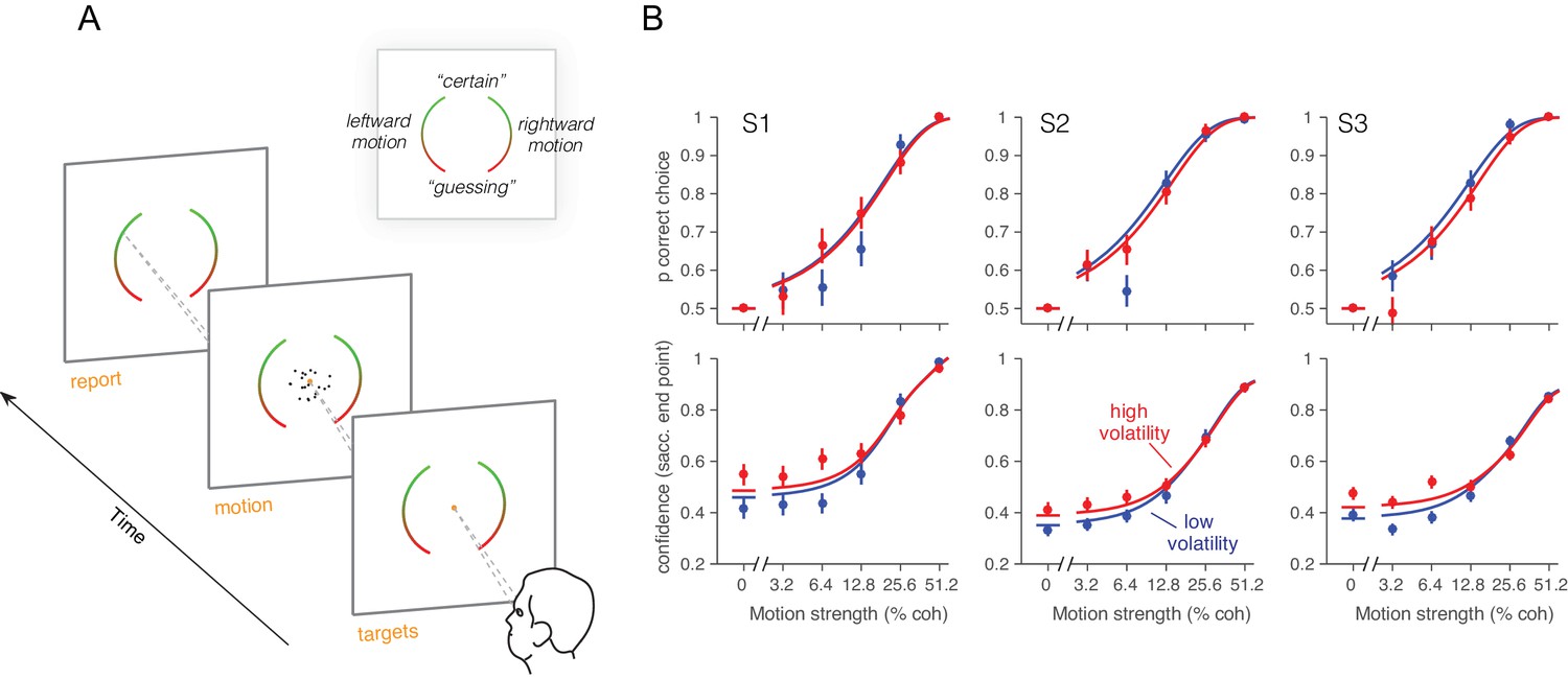
Effect of volatility on confidence rating.
(A) Task. Subjects viewed random dot motion for 200 ms and subsequently indicated a direction decision and confidence rating by looking at a left or right target (circular arc). The position along the arc indicated confidence (inset). (B) Decision confidence and accuracy. Volatility again did not affect accuracy systematically (upper panels), but the three subjects issued higher confidence ratings on trials using the high volatility display. The effect was concentrated on the weak motion strengths. Symbols are mean ± s.e.; solid traces in the upper panels are model fits in which all but one parameter were fixed by the fits in Figure 3B. Solid traces in the lower panels are predictions.
-
Figure 5—source data 1
Decision confidence and accuracy in the human confidence task.
- https://doi.org/10.7554/eLife.17688.015
Figure 6
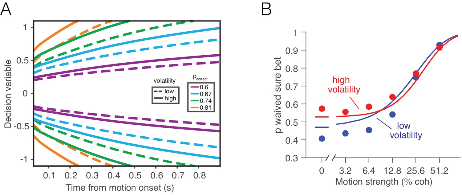
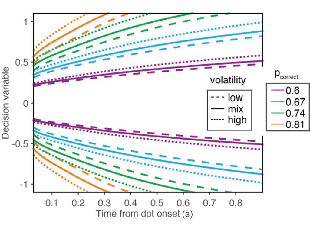
Separate mappings between the DV and confidence for high and low volatility do not explain post-decision wagering.
High and low volatility conditions would confer a different correspondence between accumulated evidence and probability correct. (A) Iso-probability contours for the probability of a correct choice under low (dashed) and high (solid) volatility. For the same stimulus duration, a larger excursion of the decision variable is required under high volatility to reach the same level of expected accuracy. (B) Probability of waiving the sure bet as a function of motion coherence, shown separately for conditions of low and high volatility. Data points are the same as in Figure 4. Solid lines represent the best fitting ‘two-map’ model, which produce visibly worse fits than the model which relies on a single, common mapping for both volatility conditions (Figure 4).
Figure 7
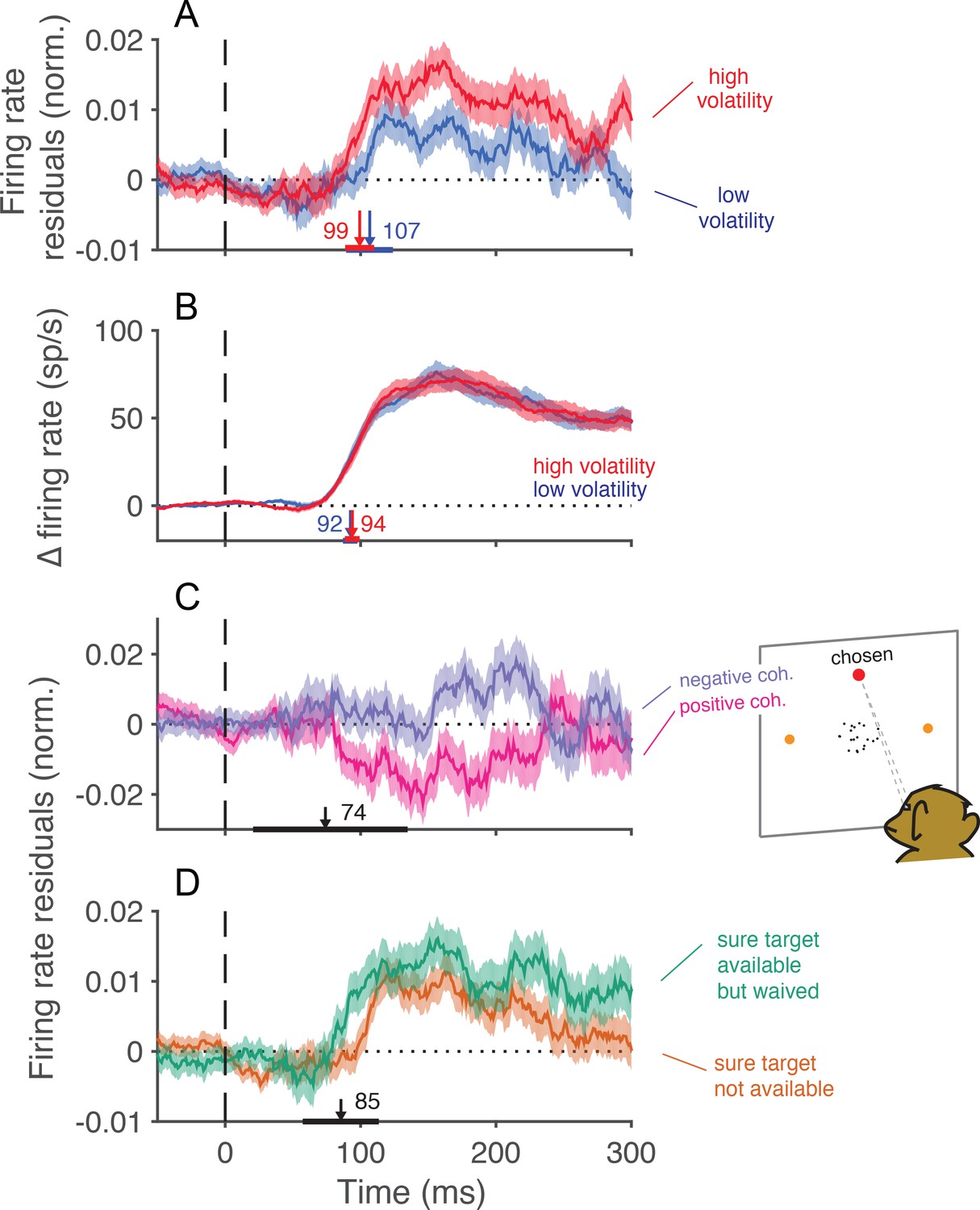
Trial-to-trial covariation between neural activity and behavior.
(A) Average of the firing rate residuals, sorted by choice. The residuals are obtained by subtracting the average response to each motion strength and direction from the smoothed single-trial response. Positive values denote higher than average activity in support of the chosen alternative. Separate averages are shown for low (blue) and high (red) volatility trials. The vertical arrows show the time when the curves first differ from baseline, estimated with a curve-fitting procedure (see Materials and methods). The associated horizontal lines are ± one standard error of the latency estimates (bootstrap). Shading shows ± 1 s.e.m. across trials. (B) Difference in firing rate between the response to the preferred and the anti-preferred direction, for high-coherence trials. Trials of low and high volatility are shown in blue and red, respectively. Error bars represent s.e.m. across neurons. (C) Average of the firing rate residuals for trials in which the sure-bet target was chosen. For statistical power, we grouped trials from both volatility conditions. Neural responses are lower than average when the correct target is in the neurons’ preferred direction (positive coherences, magenta), and above average when the motion is in the non-preferred direction (negative coherences, indigo). The arrow indicates the time at which the average residuals become significantly different from each other. (D) Average firing rate residuals sorted by choice, shown separately for trials where the sure bet was (green) or was not (orange) available. The average is greater when the sure bet was available but waived, consistent with the notion that the monkey waives the sure-bet target more often when the evidence appears to be stronger. The latency estimate (arrow) indicates the time that the difference between the curves becomes significant, which is similar to the time at which the neural activity is informative of the monkey’s choice (A).
Appendix 1—figure 1
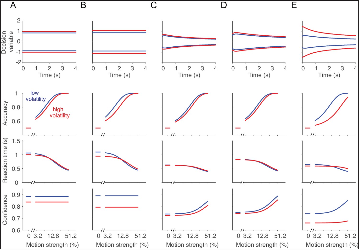
Normative decision model.
From the model comparisons we concluded that the volatility manipulation affected the noisiness of the momentary evidence without consistently affecting the parameters of the decision making process. However, it is unclear from these analyses what an optimal decision maker would do if the volatility condition were known. Therefore, we used dynamic programming to find the decision policy that maximizes average reward (Rao, 2010; Drugowitsch et al., 2012), for a variety of combinations of task parameters. The following examples are meant to convey intuitions about how parameters can change to maximize overall success per unit time. (A) Optimal solution for an experiment in which there is just one nonzero motion strength. Notice that the optimal bound height for low and high volatility trials is independent of time, consistent with a well known property of Wald’s sequential probability ratio test (Wald and Wolfowitz, 1948). The high volatility condition invites a slightly higher bound but not so much to overcome the faster decision times induced by greater noise (A, third row). Unlike the experimental observation, the normative solution assigns lower confidence under high volatility (A, bottom). (B) If the noise level associated with the high volatility condition were exaggerated further, the optimal solution would predict a greater increase in the bound height, thereby compensating for the additional noise. The bound height for the low volatility condition should increase as well. (C) In the situation we study, there are many levels of difficulty which are randomly interleaved across trials. In this situation, the optimal solution asserts a time-dependent collapse of the bounds toward lower magnitude of accumulated evidence (Drugowitsch et al., 2012). As in the single coherence case, the high volatility condition should induce an increase in bound height at all times, relative to the low volatility condition. Notice, however, that the optimal solution would lead to lower confidence under high volatility—contrary to what we observed empirically. The same pattern holds if there is a substantial time penalty after an error (D) and if the variance in the high volatility condition were exaggerated to six times that of the low volatility condition (E).
Author response image 1
Iso-confidence contours for the mappings derived from the low volatility condition, the high volatility condition, and the mixture of low and high volatilities.
The figure is similar to the new main Figure 6A, except that it also shows the map derived from the mixture of volatilities.
Author response image 2
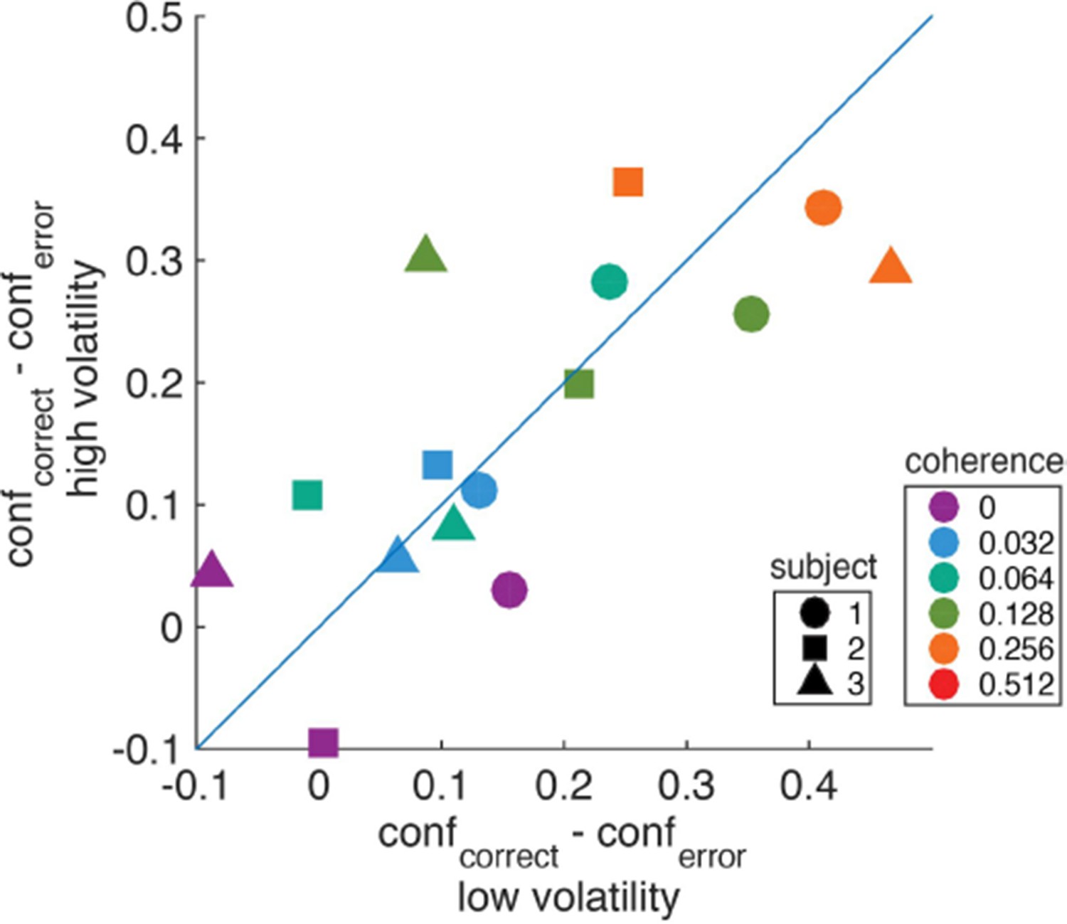
Difference in confidence (saccadic endpoint) between correct and error trials for high vs. low volatility.
https://doi.org/10.7554/eLife.17688.023
Author response image 3
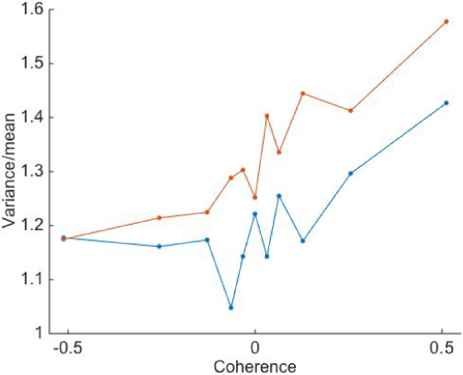
Variance-to-mean ratio of spike counts is greater under high volatility.
Trials of low and high volatility are shown in blue and red, respectively. Positive motion coherences correspond to motion in the neuron’s preferred direction. Points are averages over N=26 single neurons.
Videos
Video 1
Example motion stimuli.
The movie shows the low and high volatility examples depicted in Figure 2A. For illustration purposes, before showing the moving dots we indicate the coherence, volatility and direction of motion. These were not displayed to the participants in the experiment.
Tables
Table 1
Parameter fits for the three tasks.
| Task | RT Task | PDW | Confidence task | ||||||
|---|---|---|---|---|---|---|---|---|---|
| Subject | M1 | S1 | S2 | S3 | M2 | S1 | S2 | S3 | |
| drift rate | 10.27 | 8.64 | 12.24 | 12.69 | 10.36 | 11.84 | 18.99 | 19.06 | |
| B0 | bound parameter | 1.96 | 1.26 | 1.47 | 1.97 | 2.23 | NA | NA | NA |
| a | bound parameter | 0.64 | −2.17 | −2.63 | −2.97 | NA | NA | NA | NA |
| d | bound parameter | −0.02 | −0.26 | −0.05 | −0.23 | NA | NA | NA | NA |
| mean non-dec. time (s) | 0.28 | 0.35 | 0.34 | 0.38 | NA | NA | NA | NA | |
| stdev non-dec. time (s) | 0.06 | 0.04 | 0.02 | 0.001 | NA | NA | NA | NA | |
| conf. separatrix | NA | NA | NA | NA | 0.63 | NA | NA | NA | |
| noise scaling param. | 1.10 | 0.69 | 2.21 | 2.19 | 1.55 | RT | RT | RT | |
| noise scaling param. | 0.34 | 0.10 | 0.33 | 0.47 | 0.56 | RT | RT | RT | |
| noise scaling param. | 0.40 | 2.31 | 2.98 | 2.29 | 0.57 | RT | RT | RT | |
-
NA: not applicable; RT: values extracted from the fits to the RT task.
Table 2
Parameter fits for the alternative models.
| Task | RT Task | PDW | ||||||
|---|---|---|---|---|---|---|---|---|
| Model description | Different bound heights (B0) for high and low volatility | Two maps | Two maps, gradually | Two maps and two bounds | ||||
| Subject | M1 | S1 | S2 | S3 | M2 | M2 | M2 | |
| κ | drift rate | 10.56 | 8.71 | 10.76 | 12.31 | 10.72 | 10.40 | 10.44 |
| B0 | bound parameter | 1.77 | 1.27 | 1.47 | 1.94 | 2.24 | 2.27 | 2.92 |
| ∆B0 | bound increase, high volatility | 0.17 | −0.06 | −0.14 | 0.17 | NA | NA | -1.0495 |
| a | bound parameter | 0.72 | −1.98 | −1.97 | −2.16 | NA | NA | NA |
| d | bound parameter | 0.31 | −0.33 | −0.07 | −0.47 | NA | NA | NA |
| mean non-dec. time (s) | 0.28 | 0.35 | 0.33 | 0.37 | NA | NA | NA | |
| stdev non-dec. time (s) | 0.056 | 0.037 | 0.02 | 0.001 | NA | NA | NA | |
| ϕ | conf. separatrix | NA | NA | NA | NA | 0.626 | 0.628 | 0.629 |
| β | noise scaling param. | 1.04 | 1.11 | 0.82 | 2.37 | 1.99 | 1.60 | 1.96 |
| α | noise scaling param. | 0.673 | 0.003 | .0007 | 0.716 | 0.672 | 0.619 | 0.35 |
| γ | noise scaling param. | 0.66 | 1.76 | 1.79 | 0.94 | 0.32 | 0.415 | 0.16 |
| Speed of volatility information accrual (s) | NA | NA | NA | NA | NA | 79.36 | NA | |
| ∆BIC | Relative to base models | 29.42 | 7.7 | 27.3 | 12.1 | 252.4 | 7.24 | 126.9 |
-
NA: not applicable.
Appendix 1—table 1
Parameters explored in the normative model.
| Panel in Appendix 1—figure 1 | A | B | C | D | E |
|---|---|---|---|---|---|
| coherence set | ± 0.1 | ± 0.1 | as in the experiments | as in the experiments | as in the experiments |
| 12 | 12 | 12 | 12 | 12 | |
| 1 | 1 | 1 | 1 | 1 | |
| 1.2 | 1.4 | 1.2 | 1.2 | 2.5 | |
| (s) | 0.3 | 0.3 | 0.3 | 0.3 | 0.3 |
| (s) | 0 | 0 | 0 | 2 | 0 |
| (s) | 3 | 3 | 3 | 3 | 3 |
Download links
A two-part list of links to download the article, or parts of the article, in various formats.
Downloads (link to download the article as PDF)
Open citations (links to open the citations from this article in various online reference manager services)
Cite this article (links to download the citations from this article in formats compatible with various reference manager tools)
The influence of evidence volatility on choice, reaction time and confidence in a perceptual decision
eLife 5:e17688.
https://doi.org/10.7554/eLife.17688


