Lognormal firing rate distribution reveals prominent fluctuation–driven regime in spinal motor networks
- University of Copenhagen, Denmark
Figures
Figure 1
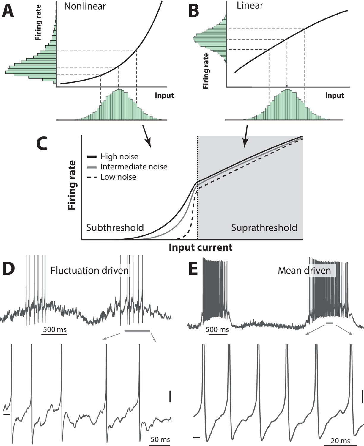
Skewness of the rate distribution reveals two regimes of neuronal spiking.
(A) In the fluctuation–driven regime the mean input is below the spiking threshold and the IO-curve has a nonlinear shape. A normally distributed input current (shown below x–axis) is transformed into a skewed firing rate distribution (y-axis). (B) In contrast, if the mean input is above threshold, the transformation is linear and the firing rate distribution is symmetric. (C) IO–function for both regimes: Linear for suprathreshold region and nonlinear for subthreshold region. The noise level affects the curvature of the nonlinearity (3 curves illustrate different levels of noise). (D) Sample recordings during motor activity from two spinal neurons in the subthreshold region, where the spiking is irregular and driven by fluctuations, and the supra–threshold region (E), where the mean input is above threshold and spiking is regular. Highlighted area shown at bottom. Spikes in bottom panel are clipped. Tick marks: −50 mV, scale bars: 5 mV. (A–B) adapted from (Roxin et al., 2011).
Figure 2 with 2 supplements
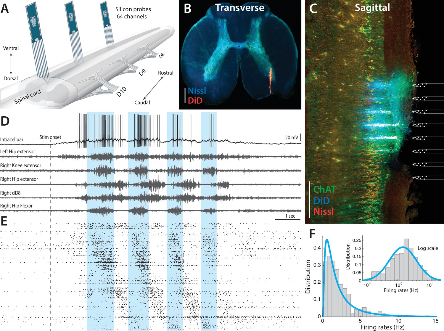
Parallel neuronal activity in the lumbar enlargement during rhythmic motor activity.
(A) Illustration of experiment with three silicon probes inserted into the lumbar spinal cord of a turtle. Histological verification: transverse (B) and sagittal (C) slices, 200 μm thick, showing the location of the silicon probes in the spinal cord (red traces and location illustrated on right, electrodes stained with DiD). ChAT staining in green and Nissl stain in blue. Scale bars: 500 μm (D) of a single neuron (top) concurrently recorded with five motor nerves (traces below) during scratching behavior induced by a somatic touch (onset indicated, 10 s duration). (E) Rastergram showing the parallel-recorded single units (200 neurons) sorted according to hip flexor phase. (F) Firing rate distribution is positively skewed and normally distributed on a log–scale, i.e. lognormal (inset). resting level in (D) is −60 mV. For details, see Figure 2—figure supplement 1 and 2.
Figure 2—figure supplement 1
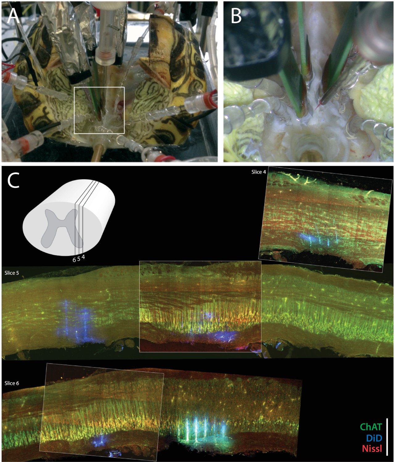
Experimental setup.
(A) Preparation with electrodes inserted into the spinal cord of a turtle, which is lying on its back with the caudal part of the carapace and spinal cord intact. The scratch reflex motor pattern is activated by the mechanical touch of the carapace with a rod attached to an actuator. (B) Close–up from (A) with nerve suction electrodes (with silver wires), an intracellular electrodes and the 3 silicon probes (green) inserted into the spinal cord. (C) Post–hoc histological reconstruction of the location of three Berg64–probes. The tissue is immunostained for ChAT-positive motoneurons (green) and Nisslstained neurons (red) to differentiate motoneurons from interneurons. The probes were painted with DiI prior to insertion leaving a fluorescent trace (blue), although unspecific ChAT staining at the shank location gives a cyan appearance in slice 6. Inset illustration indicates parasagittal locations of slice 4, 5 and 6. Scale bar: 500 μm.
Figure 2—figure supplement 2
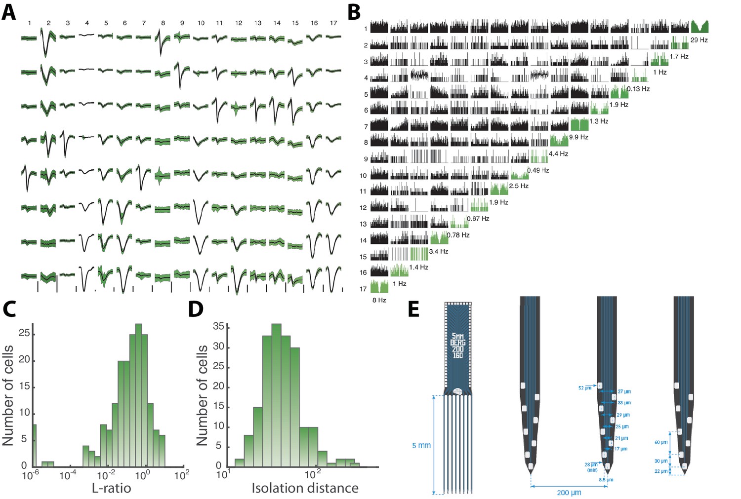
Sorted sample units, quality measures, and probe layout.
(A) Average waveforms (black) and SD (green) of 17 units (columns) recorded by 8 electrodes (rows) situation on the same shank of a Berg64–probe. Vertical scale bar 100 μV. (B) Correlogram matrix for the same 17 units with the autocorrelograms in diagonal (green). The quality of the spike sorting is verified by the L-ratio (C) and Isolation distance (D) for all units from the same session. (E) The Berg64–probe (Neuronexus inc) consists of 8 shanks with 8 electrodes on each shanks, located at the edge to sample over the largest volume of tissue. Dimensions are indicated.
Figure 3 with 2 supplements
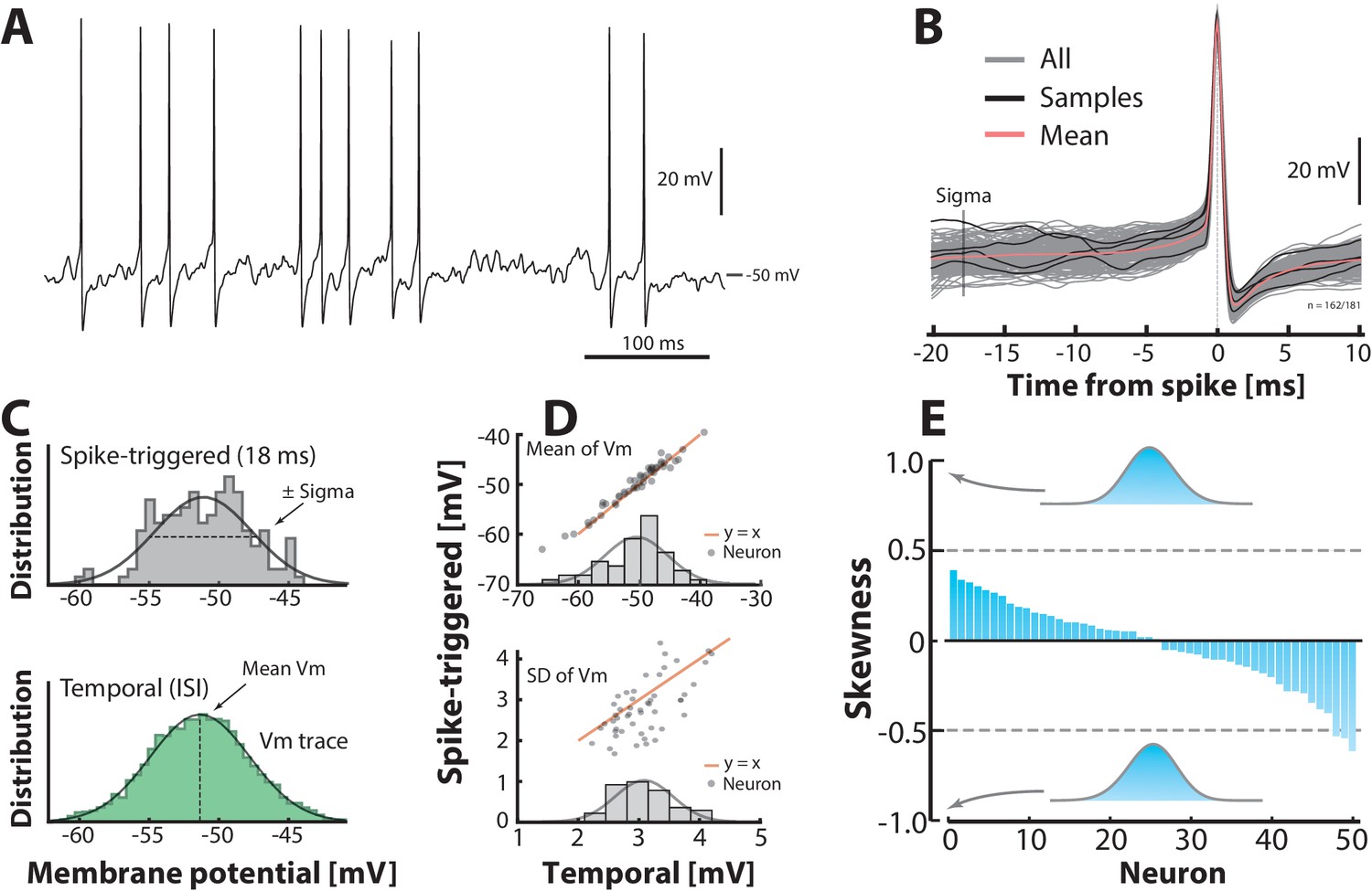
Subthreshold –distributions are symmetric.
(A) Sample cell spiking in the fluctuation–driven regime, and (B) its spike–triggered overlay to determine the –distribution of trajectories 18 ms prior to spike–onset (‘sigma’). (C) The –distribution is estimated in two ways: via samples of –instances prior to the spike peak (top, vertical line ‘sigma’ in B) and over time via the interspike intervals (bottom). (D) Mean temporal– vs. spike–triggered–estimates (top) are closely related (orange unity–line) and have a near normal distribution of means (inset). For details, see Figure 3—figure supplement 1 and 2. Similarly, the variability of the two estimates (SD) are closely related (bottom). (E) Sorted skewness for all neurons in fluctuation–driven regime indicate symmetric –distributions (temporal). Inset distributions with skewness of illustrate no discernible asymmetry. The extreme skewness observed in the data set is around 0.5 (broken lines).
Figure 3—figure supplement 1
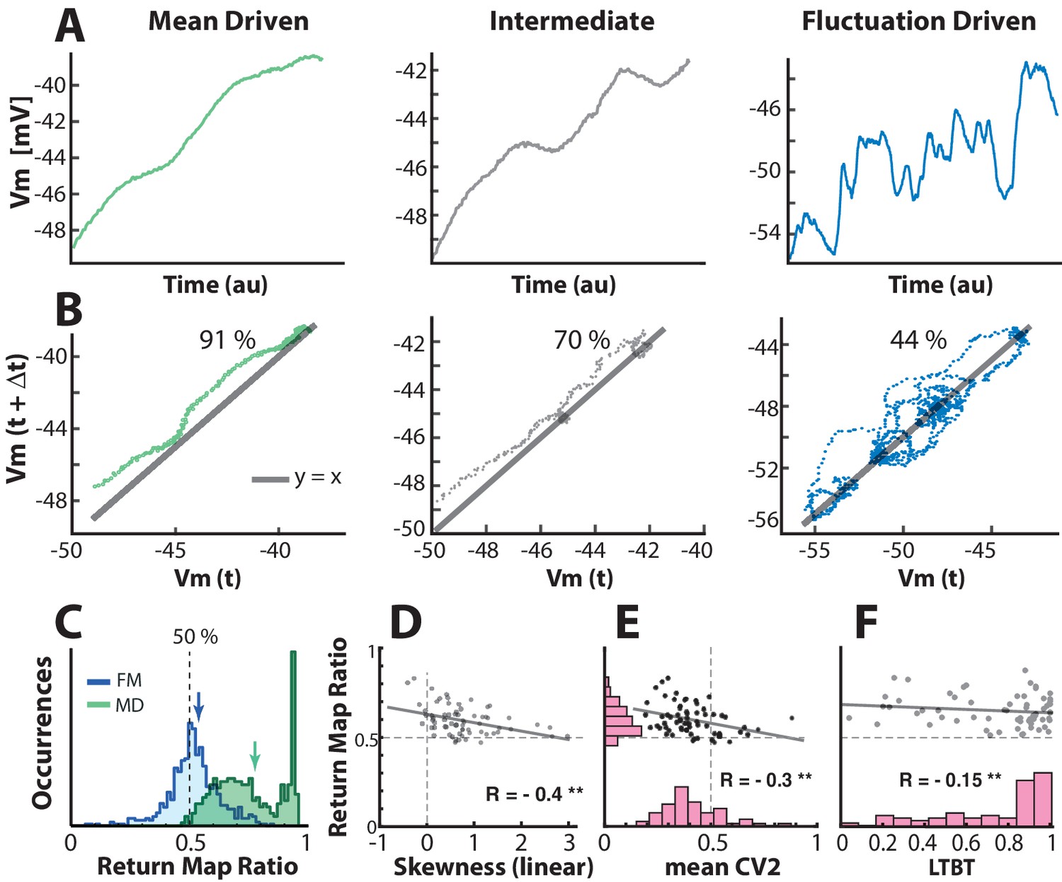
Quantifying the degree of fluctuations and selecting neurons in fluctuation–driven regime using the return map ratio metric.
(A) The inter–spike –trajectory of three sample neurons in mean–driven (left), intermediate (middle) and fluctuation–driven spiking regime (right). In the mean–driven regime the inter–spike trajectory moves directly from AHP resetting towards threshold, whereas in the fluctuation–driven regime the trajectory is convoluted and indirect (right). (B) The degree of convolution in the trajectory can be quantified using return mapping , i.e. plotting versus , and quantifying the fraction of points above versus below the unity-line (), which we refer to as the return map ratio . An even ratio close to 0.5 represents convoluted path (right), whereas a uneven ratio (close to 1) represent a direct path (left). Ratios are indicated in%. (C) The distribution of return map ratios for all ISIs, shown for two sample neurons, one having distribution mean close to 0.5, i.e. a fluctuation–driven regime and one having the mean close to 0.8, i.e. in the mean–driven regime (blue and green arrows). The mean return map ratio of all neurons () has a significant anti–correlation with skewness of firing rate distribution (D), spike irregularity () (E), as well as the least time spent below threshold (LTBT) of (F).
Figure 3—figure supplement 2

Population–distribution of mean is Gaussian.
(A) The mean for the population of neurons is symmetrically near Gaussian–distributed (blue). The mean threshold for the same population is depolarized (red). (B) The mean thresholds correlate with the values of mean and the thresholds are more depolarized as indicated by a rightward shift compared with the unity line (red). (C) Scatter plot of all the histograms of with Gaussian fits (red). (D) Histogram of the distributions with the individual mean thresholds () subtracted (broken line indicates the relative location of ). Note that the distributions, which have their mean far from threshold, also have a larger SD. (E) Normalizing each distribution with SD () to assess the distance in terms of the size of fluctuations, i.e. . (F) Scatter plot of all the distributions of , has a near Gaussian distribution as indicated with the sliding population mean (blue). The mean distance to threshold is approximately 3 (arrow).
Figure 4
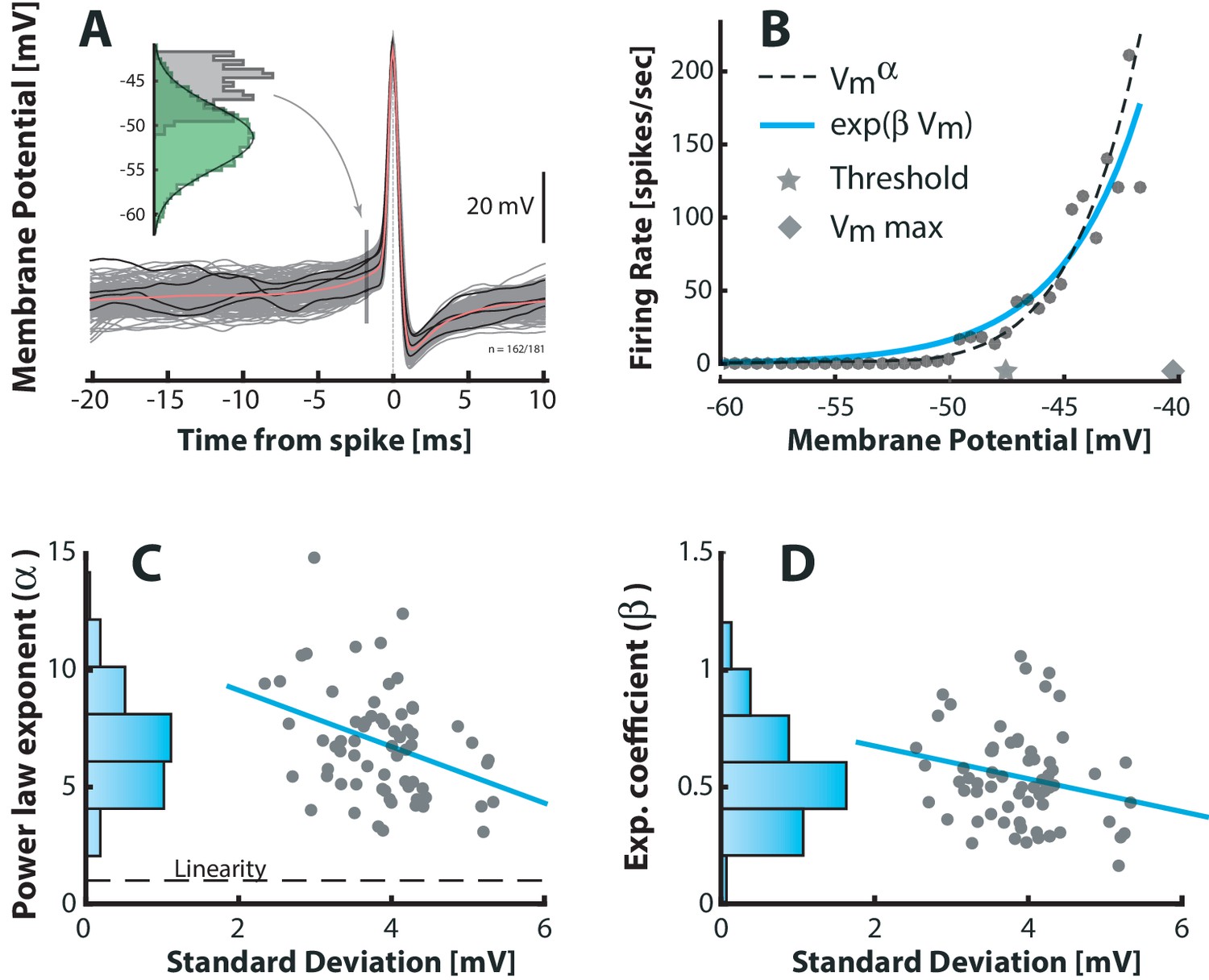
Fluctuation–driven spike–response curve is supralinear.
(A) The empirical probability of evoking a spike in a small window as a function of is determined using spike–triggered overlays. The probability distribution is estimated as the –distribution of trajectories prior to spike–onset (gray histogram, 1.7 ms prior to peak) normalized with the total (temporal) –distribution (green histogram). Dividing this probability by the sampling interval gives the firing rate (see Materials and methods). (B) The firing rate versus for a sample neuron is strongly nonlinear. A power–law (broken line) and an exponential (blue line) are fitted to capture the nonlinearity. Note that the mean threshold () is below the largest subthreshold fluctuation (), likely due to a depolarization of threshold associated with a higher firing rate (see also Figure 6—figure supplement 1). (C) Power–law exponent () for different neurons are weakly anti–correlated with the fluctuations (SD) in their (‘sigma’, Figure 3B, , p<0.01). Linearity is indicated by horizontal broken line. (D) Exponential coefficient () for different neurons are also anti–correlated with the fluctuations in albeit not significantly (, p>0.05).
Figure 5
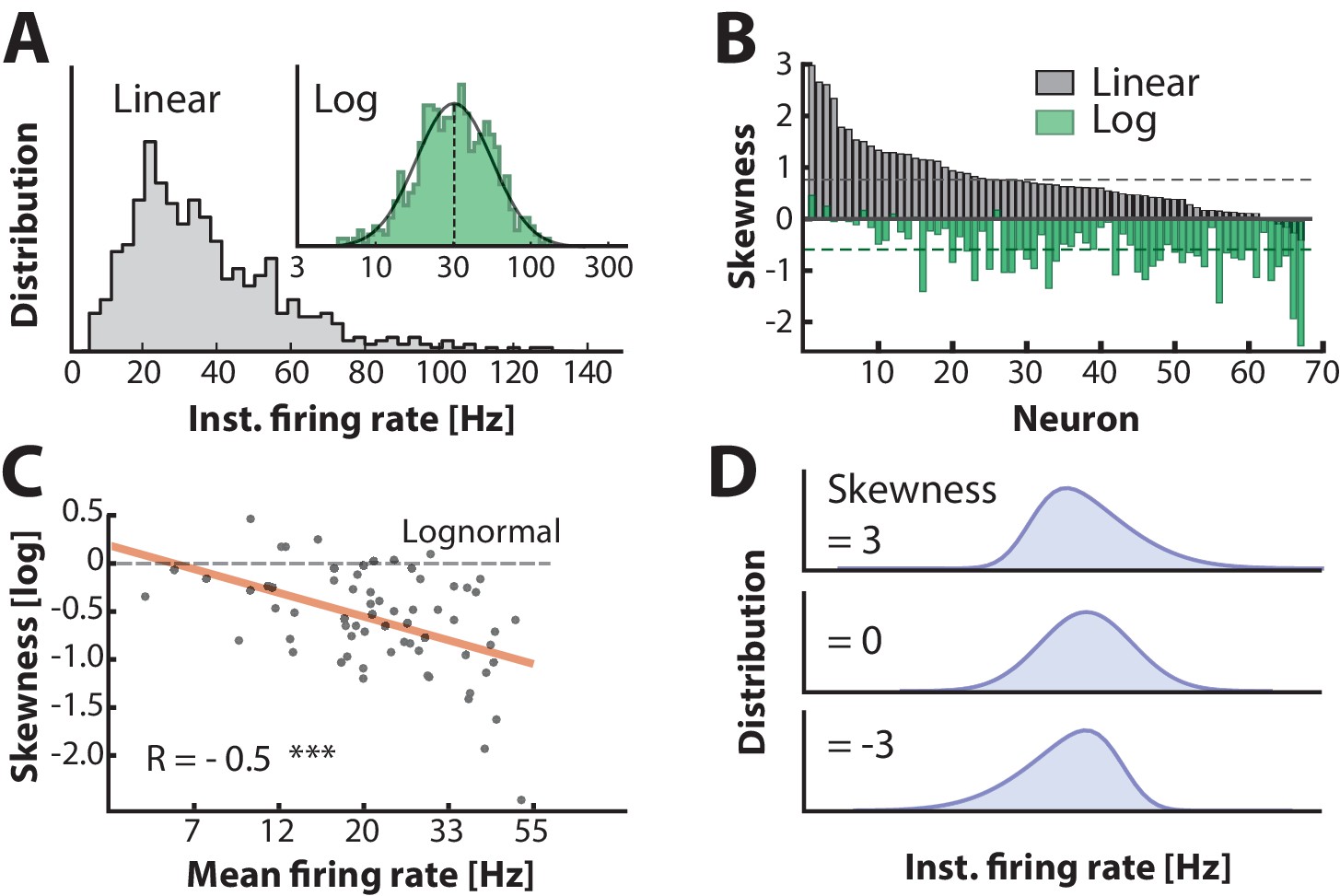
Firing rate distributions are skewed to a variable degree depending on mean firing rate.
(A) Distribution of instantaneous firing rates for a sample neuron is positively skewed on a linear axis and lognormal–like (green histogram, inset). Mean indicated by broken vertical line. (B) Sorted distribution skewness on linear (gray) and logarithmic axes (green) for each neuron in the population. (C) The log–skewness across neurons is negatively correlated (, p<0.001) with mean firing rate, which indicates that higher firing rates are found in the mean–driven regime and less lognormally–distributed, i.e. departing from broken line. (D) Illustration of firing rate distributions that have positive skewness (top), zero skewness (Gaussian, middle) and negative skewness (bottom) representing the range observed in the data (B).
Figure 6 with 1 supplement
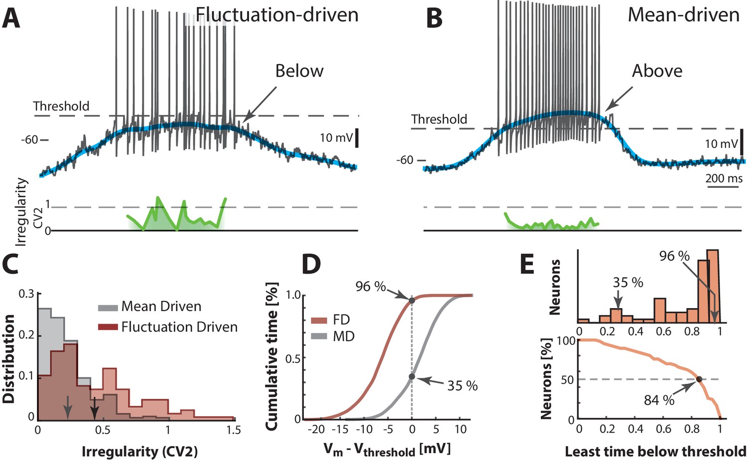
Two contrasting sample neurons found in the two regimes.
(A) Sample neuron in fluctuation–driven regime, where the mean (blue line) is below lowest threshold (broken line), the spikes are irregular (0.5–1, green line) and driven by fluctuations (arrow). (B) Second sample cell found in mean–driven regime, where the mean is above threshold during the cycle (arrow). The spiking is more regular, i.e. low (green line). (C) Mean–driven neuron (gray) has lower than the fluctuation–driven neuron (brown). Means indicated (arrows). (D) Cumulative time of shows the fluctuation–driven neuron (FD) spends more time below threshold (96%) than the mean–driven (MD, 35%). (E) Top: Time below threshold for population of neurons (cells from A–D indicated). Bottom: Least time spent below threshold versus a given fraction of neurons (reverse cumulative distribution function). Half of the neurons (broken line) spend at least 84% of the time in fluctuation–driven regime, i.e. have below threshold.
Figure 6—figure supplement 1
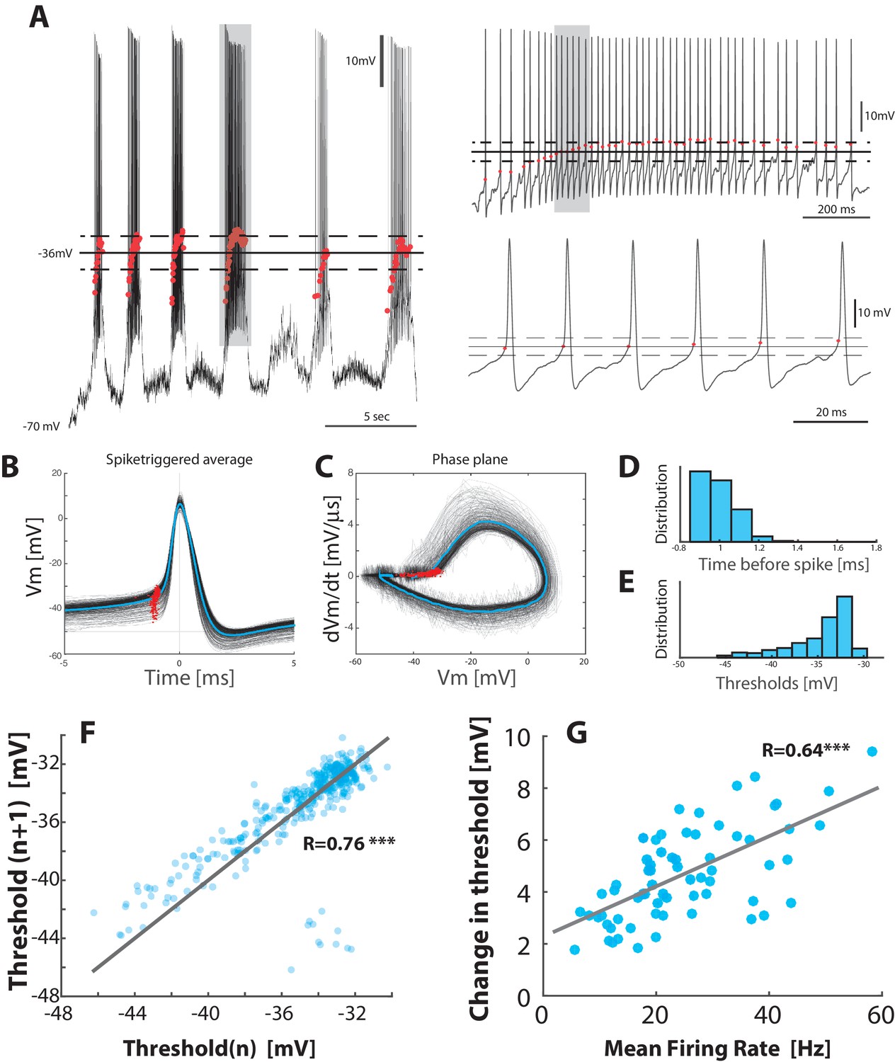
Threshold depolarizes with increase in firing rate.
(A) Sample recording with the threshold (red dots) for each spike (left). Mean threshold (solid line) SD (broken lines). Right top: the selected cycle from trace in left (fourth cycle indicated by gray horizontal bar at top). Right bottom: Selected region on shorter timescale (gray rectangle from top trace). (B) Spike–triggered overlay with the thresholds indicated (red dots). (C) Detection of threshold via method by Sekerli et al. (2004): Threshold is found at the maximum of the second derivative of the trajectory in phase plane plot of versus (red dots). (D) Distribution of threshold location prior to spike peak. (E) Distribution of threshold values in . (F) Return map of the spike threshold values, shows a strong correlation between neighboring threshold values ( vs. ). (G) The change in threshold, , with mean firing rate, where is the threshold at the 5% quantile and is the threshold for individual spikes.
Figure 7
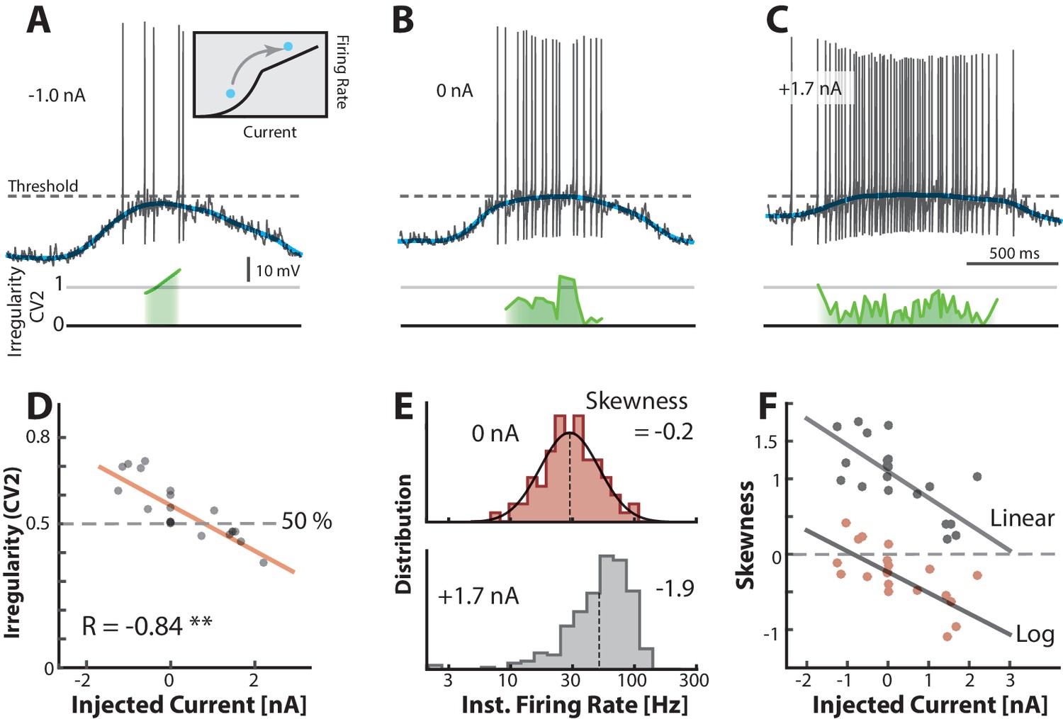
Transition between regimes can be induced by injected current.
(A) Hyperpolarizing of a sample neuron during the motor cycle with negative injected current (−1.0 nA). Negative current hyperpolarizes mean (blue) and increases irregularity (1, green line) compared with control condition (B). (C) Positive current injection (1.7 nA) has the opposite effect: Depolarization, more regular spiking and higher firing rate. (D) Mean of over a trial vs. the constant injected current for that trial has negative correlation. (E) Firing rate is lognormally distributed in control (top), but negatively skewed (skewness = −1.9) when added current increases mean–driven spiking (bottom). (F) Skewness of firing rate distribution is negatively correlated with injected current. Linear skewness shown in top gray points (, p<0.001) and log-skewness shown in bottom red points (, p<0.001). Same neuron throughout.
Figure 8 with 1 supplement
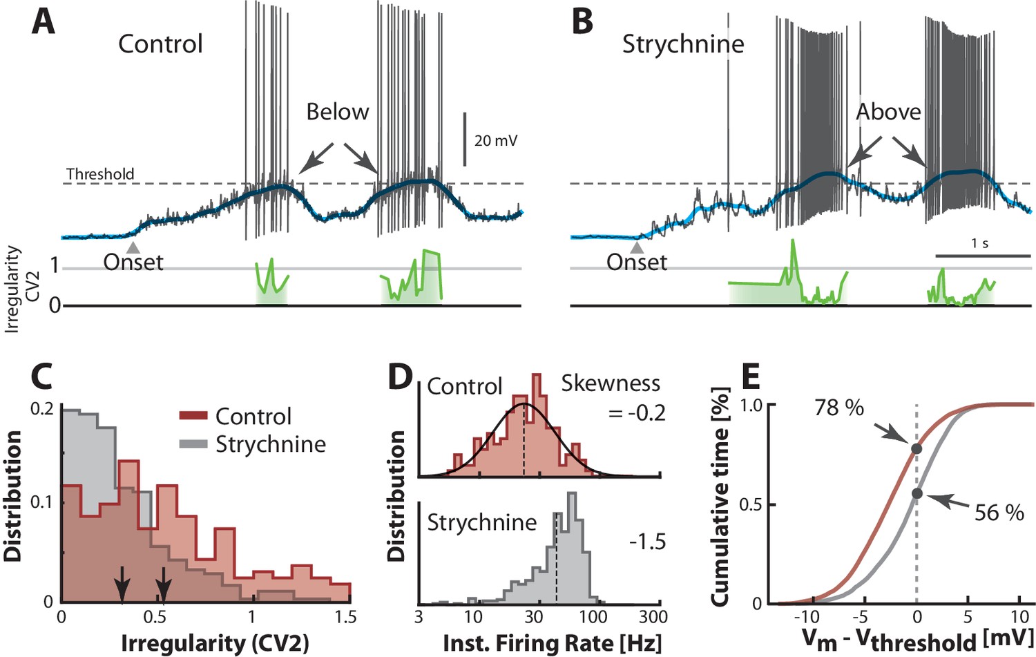
Transition between regimes induced by unbalancing E/I.
(A) Sample cell in control condition and after reduction of inhibition with local strychnine (B). Onset of motor program indicated (). Blocking inhibition results in a larger net inward current, which drives the mean (blue lines) across threshold to more mean–driven regime. As a result the spiking is less irregular on the peaks as measured with (cf. green lines). (C) Irregularity () was smaller after application of strychnine (arrows indicate mean, histogram truncated at 1.5). (D) Firing rate distribution is symmetric on log–scale (top, skewness = −0.2) and negatively skewed when inhibition is blocked (bottom, skewness=−1.5). (E) Strychnine induces a more depolarized Vm and a lower cumulative time spend below the threshold (compare 78% with 56%). Same neuron throughout.
Figure 8—figure supplement 1
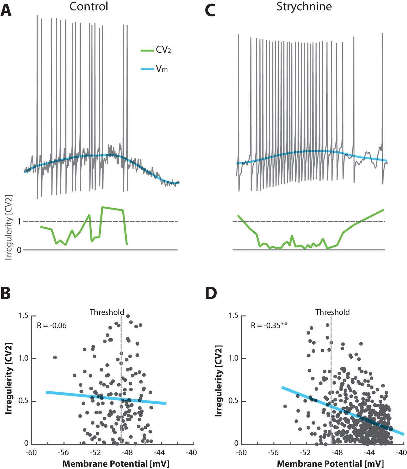
Unbalancing E/I induces an anti–correlation between irregularity and depolarization.
(A) No obvious relationship between mean (blue) and the irregularity of the spike (, green) in the control condition of a sample cell in the fluctuation–driven regime. (B) The fluctuation–driven regime is manifested as a lack of significant correlation between irregularity for each pair of ISIs () and the mean (, p=0.48). The most negative threshold indicated by vertical broken line. (C) Spiking of same cell as in (A) after elimination of glycinergic inhibition by local application of strychnine, which causes depolarized in , more regular spiking at higher rate and slower fluctuations in . (D) The removal of inhibition also puts the spiking into the mean–driven regime, which is manifested as a significant anti-correlation between irregularity of the spiking and mean (, ).
Figure 9

Skewed neuronal participation across behaviors.
(A–B) Two distinct motor behaviors: Ipsilateral pocket scratch (left panel) and contralateral pocket scratch (right panel) shown by intracellular recordings (top) and motor nerve activities. (C–D) Rastergrams showing the unit activities during ipsilateral pocket scratch (C) and contralateral pocket scratch (D). Green areas mark the hip flexor phase. (E–F) spike count firing rate distribution for the behaviors on linear and a semi-log plot (insets), indicate lognormal participation. Lognormal functions are fitted (solid green lines). (G) Skewness on logarithmic (green bars) and linear scale (gray bars) is preserved across animals. (H) The inequal neuronal participation is calculated using Lorenz curve and gini coefficient. (I) Gini–coefficients cluster around 0.5 across behaviors and animals. Mean (J) and standard deviation on (K) of the distribution of firing rates on log–scale across behaviors and animals. resting level in (A–B) is −60 mV.
Figure 10 with 1 supplement
Skewness and irregularity across the neuronal population gauge occupation in both regimes across time.
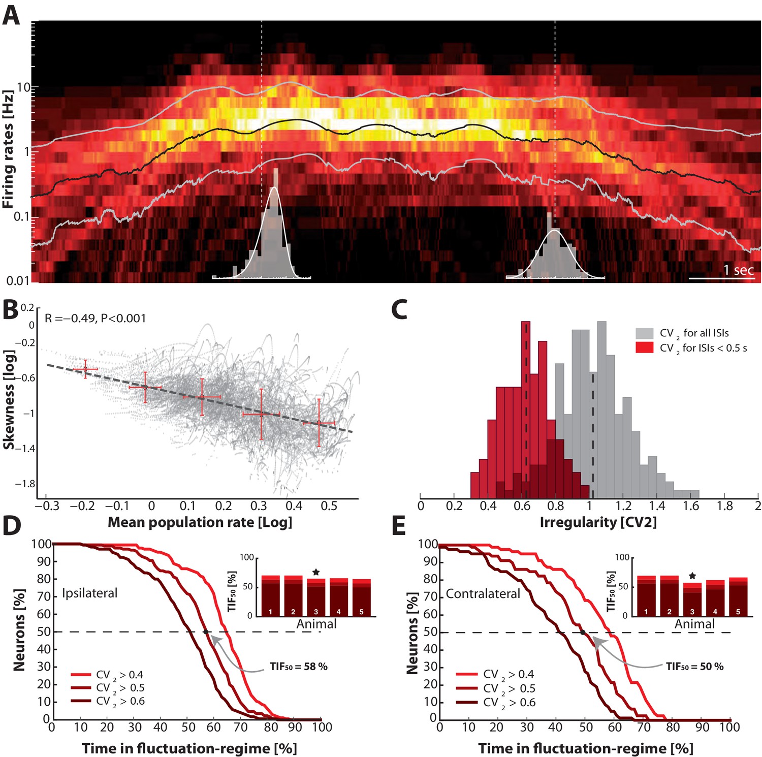
(A) Heat map of the distribution of firing rates across the population ( units, 1 animal) on log–scale (y–axis) as a function of time (x–axis). Lognormal mean SD are indicated as black and grey lines, respectively. Distribution is indicated (gray histograms) at two different time points (broken vertical lines). (B) Lognormal mean population firing rate (black line in A) versus log–skewness are negatively correlated, indicating more neurons move into mean–driven regime as the population rate increases. Scatter due to multiple trials, which is binned in sections, red crosses. (C) Distribution of irregularity (mean ) across population for all ISIs (gray) and when excluding of inter–burst intervals (red). (D) Fraction of neurons, which spend a given amount of time in fluctuation–driven regime ( and ) normalized to 100% (Reverse cumulative distribution). The least time spent in fluctuation–driven regime by half of the neurons () is given by the intercept with the broken horizontal line and distribution (indicated by arrow). For this sample animal and behavior . Inset: Values across animals, sample animal indicated (). (E) The –values across animals in both behaviors as indicated by similarity in values are remarkably conserved.
Figure 10—figure supplement 1
Distribution of neurons having fluctuation driven spikes and values.
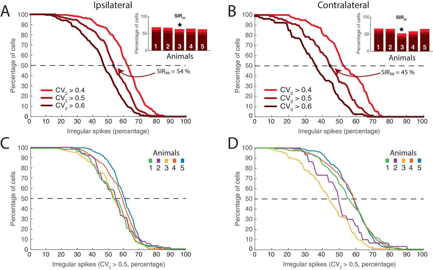
(A) Reverse cumulative distribution of neurons (y–axis) having a given number of spikes driven by fluctuations (x–axis) for ipsilateral scratching for a sample animal and three values of (0.4, 0.5, and 0.6). The minimal fraction of spikes driven by fluctuation in half of the neuronal population, , shown in inset. Sample animal indicated (). (B) Same as (A) but for contralateral scratching. (C) The reverse cumulative distributions similar to (A) for all five animals and for for ipsilateral scratching and for contralateral scratching (D).
Figure 11

Spiking irregularity is independent of cellular location.
(A) Layout of the 8 electrodes on a shank, which span a total of 210 μm in the dorsoventral axis. (B) Recorded waveforms at different locations of three sample units (colored in red, blue and green). The node locations are estimated via trilateration and indicated as rings. Electrode locations are indicated as black dots. (C) Composite of source-locations for all shanks and all animals (total cells). The location of sample units from B indicated in colors. (D) Irregularity of the associated spiking are estimated (mean on x-axis) versus the dorsoventral location (y–axis), where the unit locations are corrected for the depth of the individual shank with respect to the spinal cord surface. (E) The binned distributions of as a function of depth. The distribution means are remarkably similar (broken line as fiducial) and a KS–test indicates no significant difference.
Author response image 1
Author response image 2
Author response image 3

Author response image 4
Videos
Video 1
Skewness of the population firing rate is activity–dependent: Behavior 1 (ipsilateral scratching).
The spiking activity in three lumbar segments shown as a 24 by 8 pixel-grid, with each pixel representing a recording channel (top left panels, segments D8, D9 and D10 indicated). Columns represent probe shanks (separated by 200 μm) and rows the vertical positions in the dorsoventral axis (∼30 μm between each). The light intensity of a pixel indicate the local firing rate in time estimated using Gaussian kernels. The time-dependent distribution of firing rates across the population (green histogram, top right, logarithmic x-axis) was fitted with a lognormal function (appearing here as a normal distribution) with variable skewness (solid black line). Skewness of fit on linear and log scale is shown on slider (inset). Note the dependence on overall activity. Lower panel: spike time rastergram (horizontal lines represent spiking of the neurons, which are sorted according to phase) and time is indicated with a black bar. The scratch reflex was activated at the time-point of the vertical dotted line (‘Stim onset’). Sound is the aggregate spiking activity of the population.
Video 2
Skewness of the population firing rate is less activity–dependent: Behavior 2 (contralateral scratching).
Same neuronal activity as in Video 1, except the spinal network is now generating a different behavior. The neuronal ensemble spikes at a lower overall rate, which is reflected in a weaker relationship between skewness and activity (compare with Video 1).
Tables
Table 1
Two regimes of neuronal spiking and their definition, properties and causes.
| Fluctuation–driven | Mean–driven | Key references | |
|---|---|---|---|
| Definition | (Gerstner et al., 2014; Brunel, 2000) | ||
| Properties | Lower firing rates | Higher firing rates | |
| Irregular spiking | Regular spiking | (Amit and Brunel, 1997; Shadlen and Newsome, 1998; van Vreeswijk and Sompolinsky, 1998) | |
| Lognormal/Skewed distribution | Symmetric distribution | (Buzsáki and Mizuseki, 2014) | |
| (Roxin et al., 2011; Mizuseki and Buzsáki, 2013) | |||
| Cause | Balanced E/I | Intrinsic currents, unbalanced E/I | (Bell et al., 1995; Shadlen and Newsome, 1994; Softky and Koch, 1993) |
| Synchronized excitation | (Stevens and Zador, 1998) |
Download links
A two-part list of links to download the article, or parts of the article, in various formats.
Downloads (link to download the article as PDF)
Open citations (links to open the citations from this article in various online reference manager services)
Cite this article (links to download the citations from this article in formats compatible with various reference manager tools)
Lognormal firing rate distribution reveals prominent fluctuation–driven regime in spinal motor networks
eLife 5:e18805.
https://doi.org/10.7554/eLife.18805


