Figures and data in Detecting and representing predictable structure during auditory scene analysis

Figures
Tables

4 figures and 1 table

Figures

Figure 1

Download asset Open asset

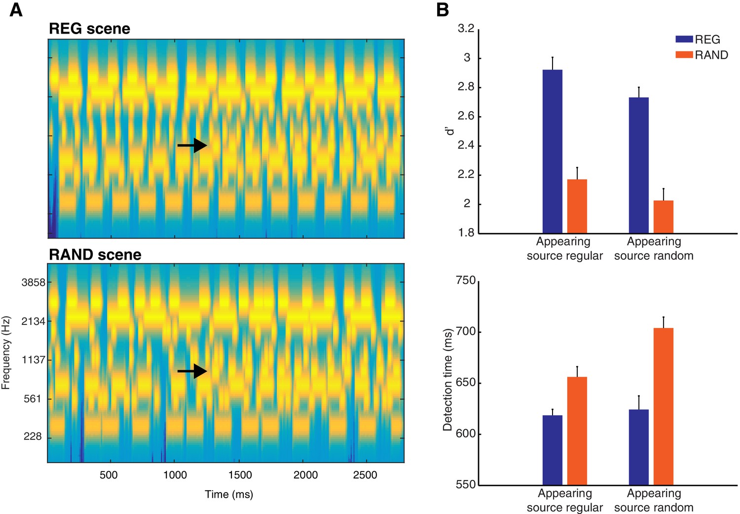
Stimuli and behavior.

(A) Examples of REG and RAND scenes. The plots represent ‘auditory’ spectrograms, equally spaced on a scale of ERB-rate (Moore and Glasberg, 1983). Channels are smoothed to obtain a temporal resolution similar to the Equivalent Rectangular Duration (Plack and Moore, 1990). Black arrows indicate appearing sources. In these examples, the appearing source is temporally regular. The stimulus set also included scenes in which the appearing source was temporally random (see Materials and methods). (B) Behavioral results (d’ and detection time) as a function of scene temporal structure (REG versus RAND). These are shown for each type of scene change (when the appearing source was temporally regular or when random). Error bars represent within-subject standard error of the mean (SEM; Loftus and Masson, 1994).

https://doi.org/10.7554/eLife.19113.003

Figure 2

Download asset Open asset

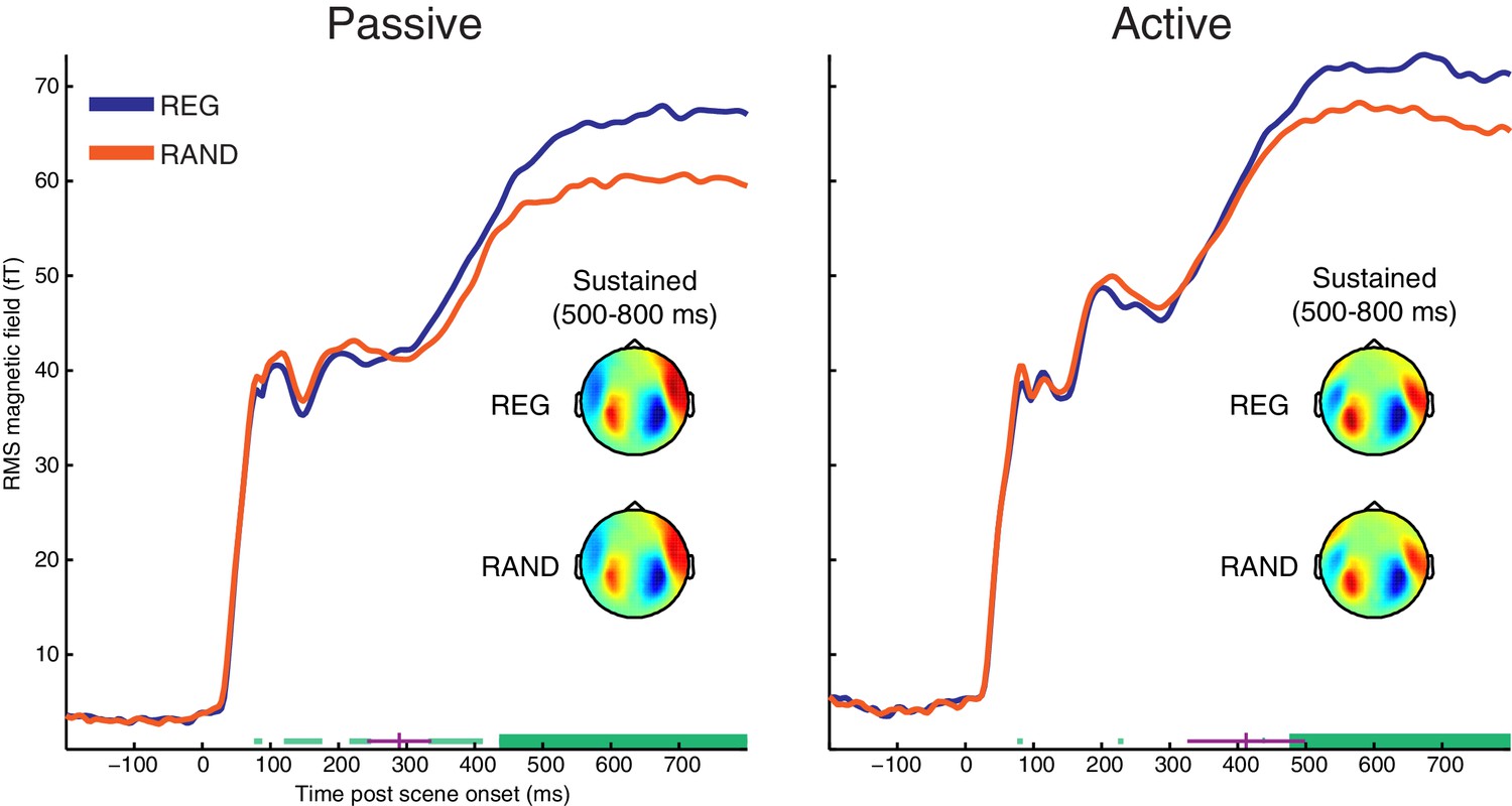
RMS time-course of the scene-evoked response showing the main effect of scene temporal structure (REG versus RAND).

Thick horizontal green lines indicate time points for which there were significant differences between REG and RAND conditions (p<0.05 FWE corrected at the cluster level; Thin light-green lines show uncorrected clusters). Purple lines indicate (jackknife-estimated) latencies of the onset of the REG versus RAND effect (horizontal and vertical portions indicate mean and jackknife-corrected standard error, respectively). Also shown are topographical patterns at the time of the sustained response (500–800 ms post scene onset), which are characterized by a dipole-like pattern over the temporal region in each hemisphere indicating downward flowing current in auditory cortex (red = source; blue = sink).

https://doi.org/10.7554/eLife.19113.004

Figure 3 with 1 supplement

Download asset Open asset

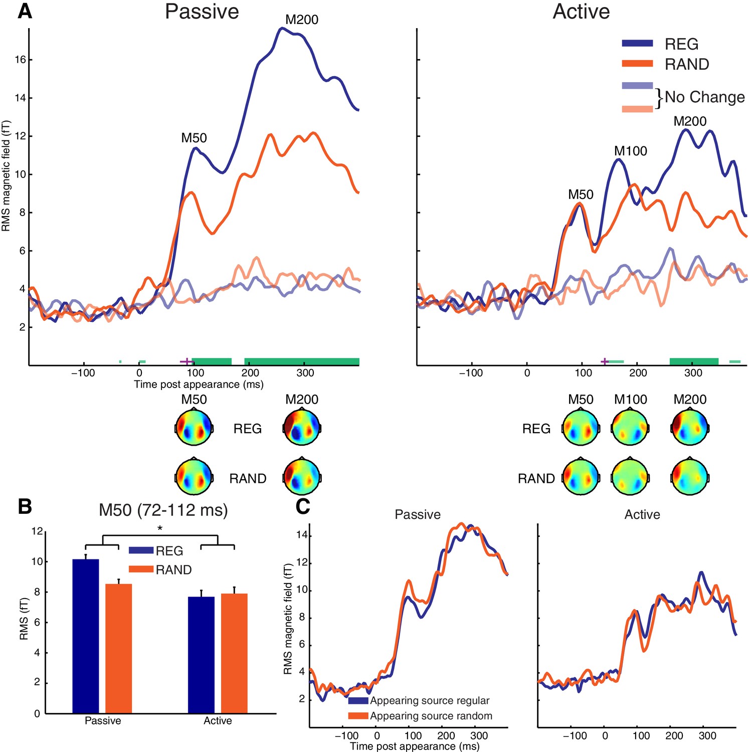
Appearance-evoked response.

(A) RMS time-course of the appearance-evoked response showing the main effect of scene temporal structure (REG versus RAND). Thick horizontal green lines indicate time points for which there were significant differences in RMS between REG and RAND conditions (p<0.05 FWE corrected at the cluster level; Thin light-green lines show uncorrected clusters). Purple lines indicate (jackknife-estimated) latencies of the onset of the REG versus RAND effect (horizontal and vertical portions indicate mean and jackknife-corrected standard error, respectively). Also shown are topographical patterns at the time of the appearance-evoked M50 (72–112 ms), M100 (144–188 ms) and M200 (232–360 ms) components. (B) Mean RMS over the appearance-evoked M50 period (712–112 ms). Asterisk indicates the significant (p<0.05) interaction ([REG>RAND]>[Passive>Active]). Error bars represent within-subject standard error of the mean (computed separately for Passive and Active groups. (C) Same as panel A but showing main effect of appearing source structure (temporally regular versus random). See also Figure 3—figure supplement 1 for the MEG time-course averaged over selected sensors responsive to the appearance-evoked M50 component.

https://doi.org/10.7554/eLife.19113.005

Figure 3—figure supplement 1

Download asset Open asset

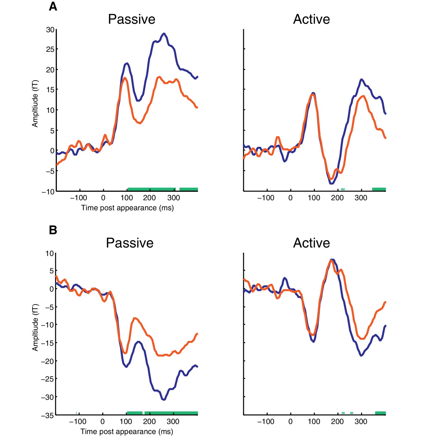
MEG time-course averaged over selected sensors responsive to the appearance-evoked M50 component.

(A) MEG from sensors showing positive signal at the time of the appearance-evoked M50 component. Thick horizontal green lines indicate time points for which there were significant differences in MEG amplitude between REG and RAND conditions (p<0.05 FWE corrected at the cluster level; Thin light-green lines show uncorrected clusters). (B) MEG from sensors showing negative signal at the time of the appearance-evoked M50 component.

https://doi.org/10.7554/eLife.19113.006

Figure 4

Download asset Open asset

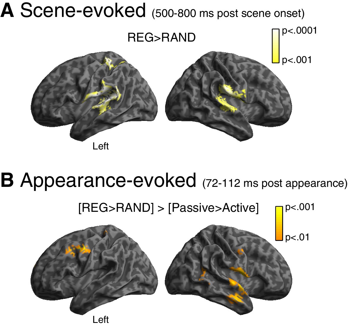
Source reconstruction.

(A) Main effect of scene temporal structure at the time of the sustained portion of the scene-evoked response (500–800 ms post scene onset). Statistical map is overlaid onto an MNI space template brain, viewed over the left and right hemispheres. Color-bar indicates statistical threshold. (B) [REG>RAND]>[Passive>Active] interaction at the time of the appearance-evoked M50 component (72–112 ms post appearance).

https://doi.org/10.7554/eLife.19113.007

Tables

Table 1

Peak voxel locations (in MNI space) and summary statistics from source reconstruction. Activations for the scene-evoked analysis are for the REG>RAND contrast (500–800 ms post scene onset) while those for the appearance-evoked analysis are for the [REG>RAND]>[Passive>Active] interaction contrast (72–112 ms post appearance). Activations have been thresholded using the same parameters as for Figure 4 (p<0.001 for scene-evoked; p<0.01 for appearance-evoked) but with an additional cluster extent threshold of n > 15 voxels (for display purposes).

https://doi.org/10.7554/eLife.19113.008

					MNI Coordinates
Analysis	Region	Side	Extent	t-value	x	y	z
Scene-evoked	Planum Temporale/Parietal Operculum	Left	1418	5.2779	−48	−28	16
(500-800 ms post scene onset)				4.364	−62	−50	14
				3.9777	−52	−30	-4
	Postcentral Gyrus	Left	204	4.8082	−32	−36	64
	Supramarginal Gyrus	Right	704	4.2469	64	−24	24
				3.7176	44	−6	16
	Planum Temporale	Right	582	3.9459	64	−16	6
				3.9252	46	−26	6
	Precentral Gyrus	Right	19	3.6051	60	6	18
Appearance-evoked	Precentral Gyrus	Left	190	3.2219	−50	−6	44
(72-112 ms post appearance)				2.9902	−34	6	38
	Precentral Gyrus/Central Operculum	Right	711	3.1966	56	0	10
				3.0153	56	4	−10
				2.9101	36	−8	16
	Middle Temporal Gyrus	Right	157	2.9859	58	−2	−24
	Middle Temporal Gyrus	Right	55	2.6951	52	−54	8
	Precentral Gyrus	Right	21	2.6444	54	−4	40
	Postcentral Gyrus	Left	16	2.5982	-30	−34	68