Divisive suppression explains high-precision firing and contrast adaptation in retinal ganglion cells
Figures
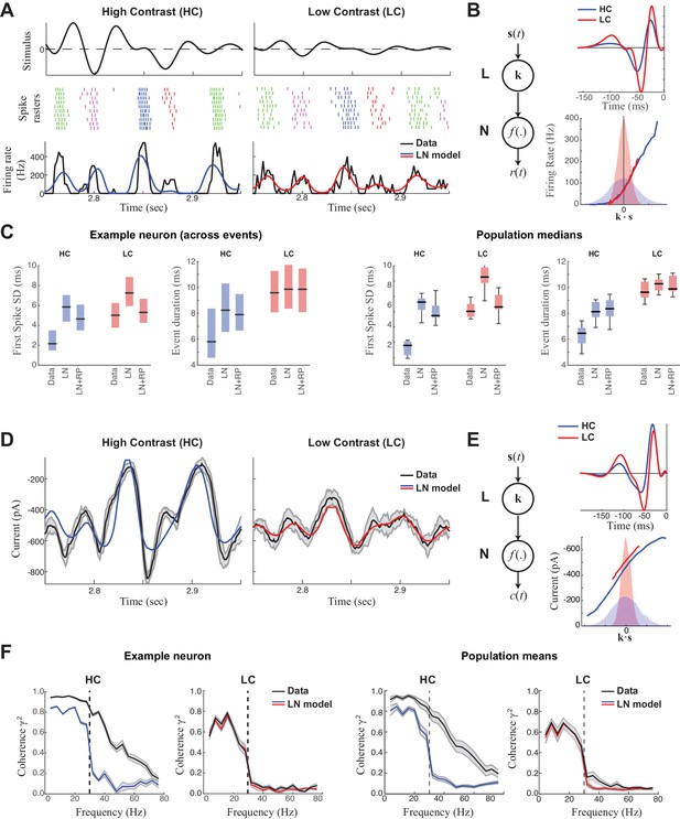
Precision of ganglion cell spike trains arises at the level of synaptic inputs.
(A) Spike rasters of an ON-Alpha cell to 10 repeated presentations of a temporally modulated noise stimulus (top) at two contrast levels. The response was parsed into separate 'events' (labeled by different colors). The PSTH (bottom) is compared with predictions of the LN model (blue, red), which fits better at low contrast. (B) The LN model (schematic: left) was fit separately at each contrast, with the effects of adaptation isolated to the linear filters (top), which share the same nonlinearity (bottom). Nonlinearities are shown relative to the distributions of the filtered stimulus at high (shaded blue) and low (shaded red) contrasts. (C) Temporal properties of the observed spike trains, compared with predictions of the LN model without or with a spike-history term (LN and LN+RP). Left: SD of the timing of the first spike in each event. Right: Event duration, measured by the SD of all spikes in the event (*p<10–6, 59 events). LN and LN+RP models do not reproduce the spike precision at high contrast (HC), but the LN+RP model is adequate at low contrast (LC). (D) Excitatory synaptic current from the neuron in (A–C) compared with the LN model predictions. Gray area indicates SD across trials, demonstrating minimal variability. (E) LN model fits to the current data. The temporal filters (top) change less with contrast compared to spike filters (Figure 1B). Note here there is also a tonic offset between contrasts (Figure 1—figure supplement 1), captured in the vertical shift of the nonlinearity (bottom right). (F). The precision of the current response was measured using the coherence between the response on individual trials and either the observed trial-averaged response (black) or LN predictions (blue, red). Gray area shows SEM across trials (left) and SD across the population (right). The LN model fails to capture high frequency response components at HC, but agrees well with the data at LC, suggesting the precision observed in ganglion cell spike trains arises at the level of synaptic inputs.
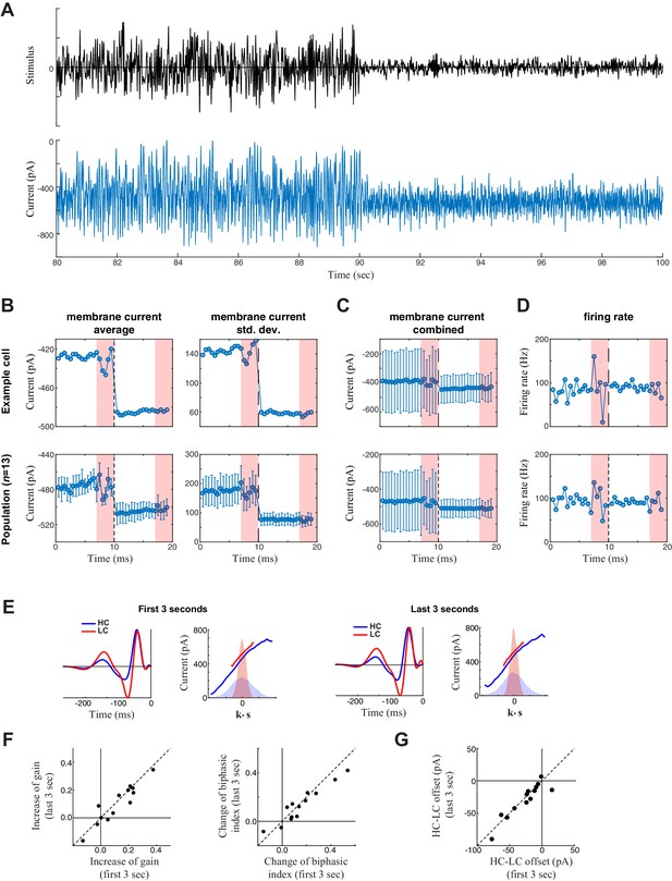
Measurement of slow contrast adaptation.
(A) The stimulus (top) and unprocessed recording of synaptic current (bottom) from an example neuron over the course of a 20 s trial consisting of 10 s high contrast (left) followed by 10 s low contrast (right). (B) Average (left) and standard deviation (right) of the membrane current over the 20 s trial for the example neuron (top) and averaged across the population (bottom). Each point is the average and standard deviation over a sliding 1 s window: each measurement was then averaged over the 10 trials. This demonstrated a tonic shift in membrane current offset (left) and gain (right) with contrast. The last three seconds of every trial represent the repeated section of the stimulus (red shaded area); the fluctuations in response to the repeated stimuli are a result of not averaging over different stimuli across the 10 trials. (C) To depict the scale of the change in mean current with contrast compared with the standard deviation (from B), the mean is represented on the same scale with the standard deviation (from B, right) with error bars extending from the averages (from B, left). The change in mean current over time was small relative to the fluctuations in synaptic current driven by the stimulus, explaining why the models did not need to incorporate mechanisms of slow contrast adaptation. The tonic shift in offset is also evident in the LN model analysis (below). (D) Average firing rate over the 20 s trial for an example neuron (top) and across the population (bottom). Each point represents the average firing rate over a sliding 1 s window across the 10 trials. The error bars in the bottom panel represent the standard deviation across the population. (E) We also tested for slower adaptation using LN analysis (e.g., Chander and Chichilnisky, 2001; see Materials and methods) based on data from the first three seconds (left) compared with the last three seconds (right) of each 7 s period of unique responses within a 10 s trial (excluding the final 3 s period of a repeated stimulus). The LN analyses for the example cell is shown. (F) Change of contrast gain (left) and biphasic index (right) across contrasts measured on the first 3 s (x-axis) and on the last 3 s (y-axis) of each trial across neurons (n = 13). We observed no difference on a cell-by-cell basis. (G) Comparison of the change in average synaptic current between contrast, comparing the first 3- and last 3 s periods, demonstrating no difference between the two periods.

Stability of recording.
To test the stability of the recording, we calculated the standard deviation of intracellular synaptic current responses (top) and average current (bottom) over the 10 trials of each experiment (box plots show data aggregated across cells, n = 13). Recordings were stable across trials.
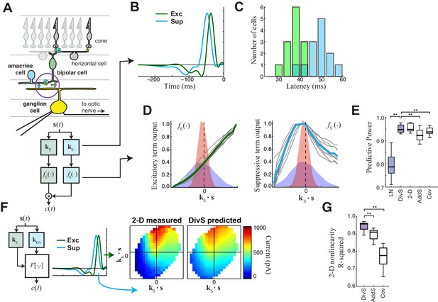
The divisive suppression (DivS) model of synaptic currents.
(A) Schematic of retinal circuitry. The vertical excitatory pathway, cones → bipolar cells → ganglion cell, can be modulated at the bipolar cell synapse by amacrine cell-mediated inhibition of bipolar cell release or by synaptic depression. We model both processes by divisive suppression (bottom), where an LN model, representing the collective influence of amacrine cell inhibition and synaptic depression, multiplicatively modulates excitatory inputs from bipolar cells to the ganglion cell. (B) The excitatory (green) and suppressive (cyan) temporal filters of the DivS model for an example ON-Alpha cell. (C) Divisive suppression is delayed relative to excitation, demonstrated by the distributions of latencies measured for each pair of filters (mean delay = 10.9 ± 2.2 ms, p<0.0005, n = 13). (D) Excitatory (left) and suppressive nonlinearities (right) for the DivS model. The solid line indicates model fits for the example cell, and the gray lines are from other cells in the population, demonstrating their consistent form. The distribution of the filtered stimulus is also shown as the shaded area for HC (blue) and LC (red). The suppressive nonlinearity (right) falls below one for stimuli that match the kernel or are opposite, implying that divisive suppression is ON-OFF. (E) To validate the form of the DivS model, we compared its performance to alternative models, including a more general model where the form of the nonlinearity is not assumed (2-D, see below), a model where excitatory and suppressive terms interact additively (AddS) instead of divisively, and a covariance (COV) model similar to spike triggered covariance (Figure 2—figure supplement 1). The DivS model performed significantly better than the LN, AddS and COV models (**p<0.0005, n = 13), and matched the performance of the 2-D model. (F) We used a 2-dimensional nonlinearity to capture any more general interaction between excitatory and suppressive filters, shown with schematic (left), and the resulting fits (middle). Consistent with the model performance (E), the form of this 2-D nonlinearity could be reproduced by the DivS model (right). (G) Accuracy of the ability of the DivS, AddS, and COV models to reproduce the 2-D nonlinearity across neurons (**p<0.0005, n = 13).
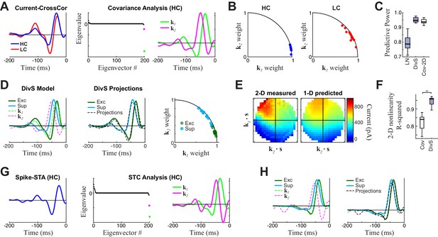
Comparison to covariance-based models.
(A–F) Covariance-based analysis of synaptic currents for the same example cell as in Figure 1. Covariance analysis follows the intuition of spike-triggered covariance (STC), but uses continuous current input rather than spikes (see Materials and methods). (A) Left: Cross-correlation between the stimulus and current response (the equivalent of a spike-triggered average) for high contrast (HC, blue) and low contrast (LC, red) stimuli. Filters are scaled to have the same standard deviation, for comparisons of shape. Middle: The eigenvalue spectrum for the response-triggered covariance matrix in HC, revealing two significant eigenvalues (color-coded). Right: The corresponding eigenvectors. (B) The locations of the cross-correlations in HC (blue, left) and LC (red, right) within the 2-D subspace spanned by the two significant eigenvectors for all neurons (n = 13). Because they are all close to the unit circle, both HC and LC cross-correlations were largely contained in the covariance (COV) subspace, consistent with previously reported results for spikes (Liu and Gollisch, 2015). (C) Model performance for the LN, DivS, and COV models (n = 13), reproduced from Figure 2E. This demonstrates that the COV filters coupled to a 2-D nonlinearity (described below) can nearly match the performance of the DivS model. (D) Left: The excitatory (green) and suppressive (cyan) filters of the DivS model, plotted in comparison to the filters identified by covariance analysis (dashed lines). Middle: The DivS model filters shared the same 2-D subspace as the covariance filters, as shown by comparing the filters to optimal linear combinations of the COV filters (black dashed), following previous work based on spikes (Butts et al., 2011). Right: The DivS filters projected into the COV filters subspace across neurons, using the same analysis as in (B). Their proximity to the unit circle shows they are almost completely in the covariance subspace for all neurons, again consistent with previous work with spikes (Butts et al., 2011). (E) Left: The 2-D nonlinearity associated with the COV filters, for the example neuron considered. Right: The best 2-D nonlinearity reconstructed from 1-D nonlinearities operating on the COV filters. Unlike the 2-D nonlinearity associated with the DivS filters (Figure 2F), this nonlinearity could not be represented as the product of two 1-D nonlinearities. (F) The separability of 2-D nonlinearities for the COV and DivS models, measured as the ability of the 1-D nonlinearities to reproduce the measured 2-D nonlinearity (R2) across neurons (**p<0.0005, n = 13). (G–H) STC analysis applied to an example neuron for which there was enough spiking data. (G) The spike-triggered average (left), eigenvalue spectrum (middle), and significant STC filters (right). (H) As with the analyses of current responses above, the DivS filters (green, cyan) did not match those identified by STC (left, dashed), but were largely contained in the subspace spanned by the STC filters (right), as shown by comparing to their projections into the STC subspace (dashed black). Note that there was not enough data to estimate 2-D nonlinearities for the spiking data, and so no comparison of STC model performances could be made.
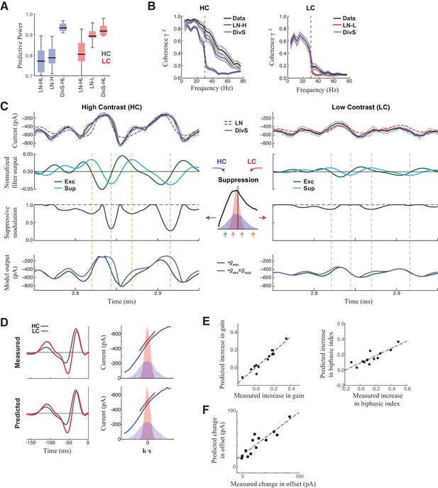
DivS model explains temporal precision and contrast adaptation in synaptic currents.
(A) The predictive power of models across contrasts. The DivS model is fit to both contrasts using a single set of parameters, and outperforms LN models fit separately to either high or low contrast (LN-H and LN-L). As expected, the LN model fit for both contrasts (LN-HL) performs worse than separately fit LN models, because the LN-HL model cannot capture the filter changes without changes in model parameters. (B) Average coherence between model predictions and recorded synaptic currents on individual trials (n = 13), shown for high contrast (HC) and low contrast (LC). The DivS model prediction performs almost identically to the trial-averaged response. (C) DivS model explains precision and contrast adaptation through the interplay of excitation and suppression. Top: comparison of predictions of synaptic current response of the LN model and the DivS model for the cell in Figure 1. second row: normalized output of the excitatory and delayed suppressive filter. 3rd row: suppressive modulation obtained by passing the filtered output through the suppressive nonlinearity (middle inset). Bottom: excitatory output of the DivS model before and after the suppressive modulation. In LC, the suppressive term (third row) does not deviate much from unity, and consequently the DivS model output resembles the excitatory input. (D) Comparison of the measured (left) and DivS model predicted (right) LN models across contrast. (E) The LN analysis applied to the DivS model predictions captures changes of both contrast gain (left: R = 0.96, p<10–6) and biphasic index (right: R = 0.86, p<0.0005) of the temporal filters across contrasts. (F) The DivS models predict the changes in tonic offset without any additional parameter shifts (R = 0.90, p<10–4).
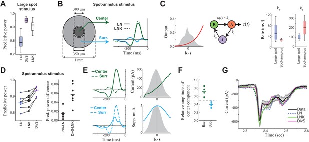
Probing the mechanism of divisive suppression with center-surround stimuli.
(A) For the large spot stimulus, the Linear-Nonlinear-Kinetic (LNK) model nearly matches the performance of the DivS model, and outperforms the LN model. (B) To distinguish between different sources of divisive suppression, we presented a spot-annulus stimulus (left), where each region is independently modulated. Model filters can be extended to this stimulus using a separate temporal kernel for center and surround, shown for the LN and LNK model filters (right), which are very similar. (C) After the linear filter, the LNK model applies a nonlinearity (left), whose output drives the transition between resting and activated states (middle), which is further governed by kinetics parameters as shown. Critical kinetics parameters for LNK models differed between the large-spot and spot-annulus stimulus (right), with the spot-annulus model very quickly transitioning from Inactive back to Active states, minimizing the effects of synaptic depression. (D) The performance of the spatiotemporal LNK model is only slightly better than that of the LN model, and neither captures the details of the modulation in synaptic current, compared with the DivS model. (E) The spatiotemporal DivS model shown for an example neuron exhibits different spatial footprints for excitation and suppression, with excitation largely driven by the spot and suppression by the annulus. This divisive suppression cannot be explained exclusively by synaptic depression, which predicts overlapping sources of suppression and excitation (Figure 4—figure supplement 1 and 2). (F) The contribution of the center component in the DivS model for excitation (left) and suppression (right). Excitation was stronger in the center than in the surround (center contribution>0.5, p=0.016, n = 7) and suppression was weaker in the center (center contribution<0.5, p=0.016, n = 7) for every neuron. (G) The DivS model captured temporal transients in the current response to spot-annulus stimuli better than the LN and LNK models.
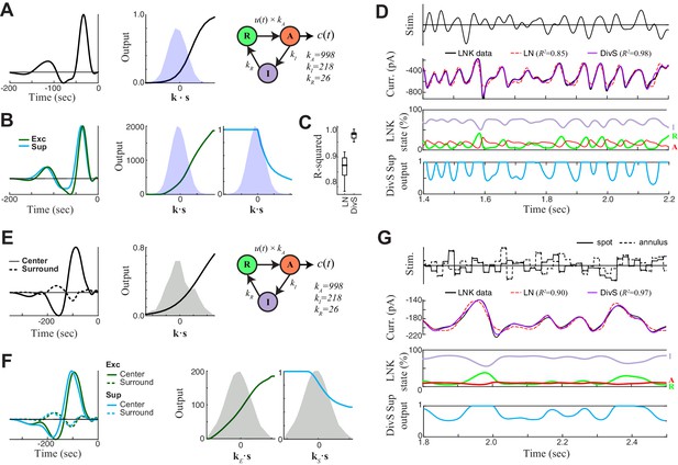
DivS model localizes the suppressive components of LNK model and reproduces its simulated response.
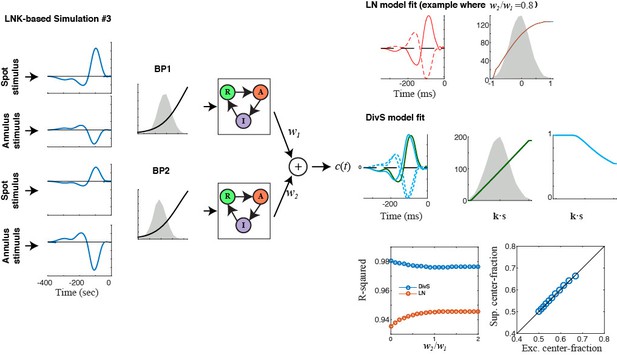
We simulated LNK models resembling the example neurons considered in Figure 4. (A–D) LNK simulation in response to a temporally modulated spot. (A) The LNK model components consist of a temporal filter k (left) and static nonlinearity f(∙) (middle), whose output u(t)=f[k∙s(t)] governs the transition rate between the resting (R) and active (A) states. The current output is proportional to active state occupation, and other constants govern the transition to inactive (I) state and back to resting state. The parameters for this LNK simulation were derived from an LNK fit to an example neuron (see Materials and methods). (B) A DivS model was fit to the LNK model simulated response, with components labeled as in Figure 2. The temporal filter of suppression (cyan) is delayed relative to the excitation (left) and only results in suppression for ON stimuli, as expected given its relationship to synaptic depression. (C) Model performance (R2) for the LN model and DivS model across all neurons demonstrates that the DivS model could reproduce LNK simulations with greater than 90% accuracy, across simulations of all LNK models of recorded neurons (n = 13). (D) Simulated response of the LNK model in (A) in response to a temporal modulated spot stimulus (top). 2nd row: The output of the LNK simulation (black) could be reproduced better by a DivS model (red) fit to the simulated data, as compared to the LN model (blue). 3rd row: The occupation of each internal state determined the current output in addition to the output of the LN component of the model. 4th row: The dynamics of the divisive suppression of the DivS model (cyan) roughly matched the occupation of the resting state of the LNK model (3rd row, green): the resting state occupancy (and availability for transition to the active state and resulting current output in the LNK model) was low at the same times there is suppression in the DivS model. (E–G) LNK simulation in response to the spot-annulus stimulus. (E) LNK components are labeled identically as in (A), but now the filter k consists of separate components for the spot (left, solid) and annulus (dashed) regions of the stimulus. The temporal filter and nonlinearity were derived from the example cell in Figure 4B, but the kinetics parameters of the temporally modulated stimulus (A) were used in place of those derived for the spot-annulus stimuli, because the latter parameters did not result in nonlinear effects. (F) A DivS model fitted to the LNK model simulated response, with components labeled as in Figure 2, resulting in the expected delayed ON suppression (as with the temporally modulated spot simulations in B). (G) Simulated response using the LNK model with the spot-annulus stimulus, again with the divisive suppression of the DivS model (4th row, cyan) capturing the occupancy of resting state of the LNK model (3rd row, green).
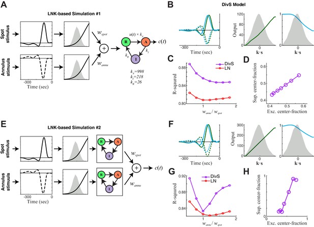
DivS model descriptions of extended LNK models.
Here we consider additional model structures involving synaptic depression. The simulations here incorporate nonlinear rectified subunits, and were limited to two components corresponding to those independently modulated in the stimulus: spot and annulus. (A–D) First we considered an extended LNK model with independent stimulus processing of the spot and annulus stimuli, and a shared synaptic depression stage. (A) Model schematic, showing that the separate 'center' and 'surround' components (corresponding to spot and annulus stimuli) are each rectified before being combined, and fed into the LNK model for synaptic depression, using the same kinetic parameters considered for simulations in Figure 4—figure supplement 1. Simulated data were generated for a range of models of this form, where the weight for the ‘spot’ component wspot was fixed and the annulus component weight wannu was varied. (B) The DivS model components fit to an example simulated response of the extended LNK model (with wspot = wannu). As with simpler circuits (e.g., Figure 4—figure supplement 1), suppression was delayed relative to excitation. Note that the DivS model was limited to only a single rectified component to match the form used to describe experiments described in Figure 4. (C) The performance of the LN (red) and DivS (purple) models across simulations with different annulus component weights. The DivS model performance was significantly better than that of the LN model over a wide range of parameters (each point corresponds to the results of simulation with different choice of wannu), suggesting a large portion of the synaptic depression effect was captured by the DivS model. Note, however, that the DivS model has a more difficult time explaining this [simulated] data than the data from real ON-Alpha ganglion cells (i.e., Figure 4D). (D) For all simulations, the 'spatial profile' of suppression matched that of excitation, as measured by the 'center fraction', which was given by the norm of the center component of the filter divided by the norm of the full filter. [The center fraction is one for no surround component, and zero for no center component.] (E–H) We next considered an extended LNK model with both independent stimulus processing and independent kinetics. (E) Model schematic, showing the separate center and surround components each with independent synaptic depression — again with the same kinetic parameters previously considered. (F) The DivS model components fit to an example simulated response of the extended LNK model (with wspot = wannu). (G) Performance of DivS model and LN model on simulated LNK model response. (H) Tight correlation of the center fractions of excitation versus divisive suppression of the DivS model components (as in panel D). This and related simulations (i.e., with additional center-surround filtering prior to the rectification stage) involving synaptic depression never yielded a case where DivS excitation was largely from the center and suppression was largely from the surround, which was observed in the real ON-Alpha cell data (e.g., Figure 4E).
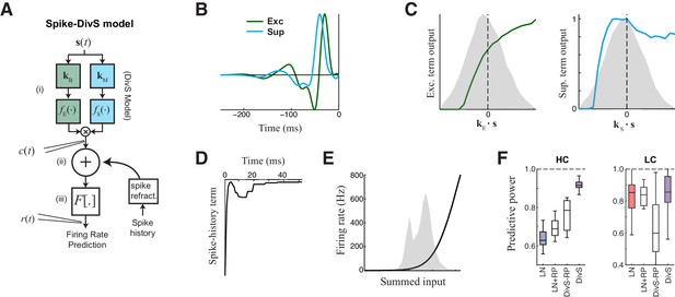
The extended divisive suppression model explains ganglion cell spike trains with high precision.
(A) Model schematic for the divisive suppression model of spiking, which extends DivS model for the current data by adding an additional suppressive term for spike-history (refractoriness), with the resulting sum passed through a rectifying spiking nonlinearity. (B–E) The model components for the same example neuron considered in Figures 1–3. (B) The excitatory and suppressive filters. (C). The excitatory and suppressive nonlinearities. The filters and nonlinearities were similar to the DivS model fit from current data (shown in Figure 2B). (D) The spike-history term, demonstrating an absolute and relative refractory period. (E) The spiking nonlinearity, relative to the distribution of generating signals (shaded). (F). The predictive power of different models applied to the spike data in HC and LC. The DivS model performs better than other models (HC: p<0.001; LC: p<0.002, n = 11), including the LN model, the LN model with spike history term (LN+RP), and a divisive suppression model lacking spike refractoriness (DivS-RP). Only a single set of parameters was used to fit the DivS model for both contrasts, whereas all other models shown used different parameters fit to each contrast.
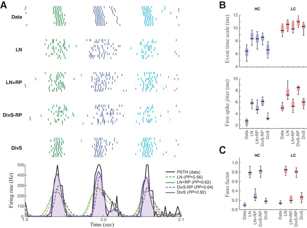
Spike patterning is shaped by a combination of nonlinear mechanisms.
(A) Top: Spike rasters recorded over ten repeats for an example cell (black) compared with simulated spikes from four models: LN, LN model with spike-history term (LN+RP), the DivS model without spike-history (DivS-RP), and the full DivS model (DivS). Colors in the raster label separate spike events across trials (see Materials and methods). Bottom: The PSTHs for each model demonstrate that suppressive terms are important in shaping the envelope of firing (DivS prediction is shaded). (B–E) Using event labels, spike statistics across repeats were compiled to gauge the impact of different model components. (B) The temporal properties of events compared with model predictions, across contrast (same as Figure 1, with DivS-based models added). Both spike-history and divisive suppression contribute to reproduce the temporal scales across contrast. (C) The Fano factor for each event is a measure of reliability, which increased (i.e., Fano factor decreased) for models with a spike-history term.
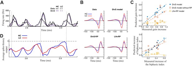
Contrast adaptation in the spike output depends on both divisive suppression and spike refractoriness.
(A) The full spike-DivS model accurately captured contrast adaptation. Top: observed PSTH and predicted firing rates of the DivS model at HC and LC. (B) The DivS model predicted the changes in LN filter shape and magnitude with contrast for an example cell. Predicted changes are shown for each model, demonstrating that the full effects of contrast adaptation require both divisive suppression and spike-history terms. (C) Measured and predicted contrast gain (top) and changes of biphasic index (bottom). The DivS model accurately predicted a contrast gain and changes biphasic index across contrast across cells (contrast gain: slope of regression = 0.75, R = 0.85, p<0.001; biphasic index: slope of regression = 0.87, R = 0.87, p<0.001). DivS model without the spike history term underestimated contrast adaptation (contrast gain: slope of regression = 0.53, R = 0.51, p = 0.10; biphasic index: slope of regression = 0.49, R = 0.73, p<0.05), and the LN+RP model failed to predict adaptation altogether (contrast gain: slope of regression = 0.06, R = 0.28, p = 0.41; biphasic index: slope of regression = −0.07, R = −0.18, p = 0.60). (D) The suppressive effect from the spike-history term was amplified at HC, due to the increased precision of the spike train. Dashed lines show the onset of HC spike events, which predict the largest difference in the magnitudes of the suppression between contrasts.
