Inhibitory control of correlated intrinsic variability in cortical networks
- University College London, United Kingdom
- MTA TTK NAP B Sleep Oscillations Research Group, Hungary
Figures
Figure 1 with 1 supplement
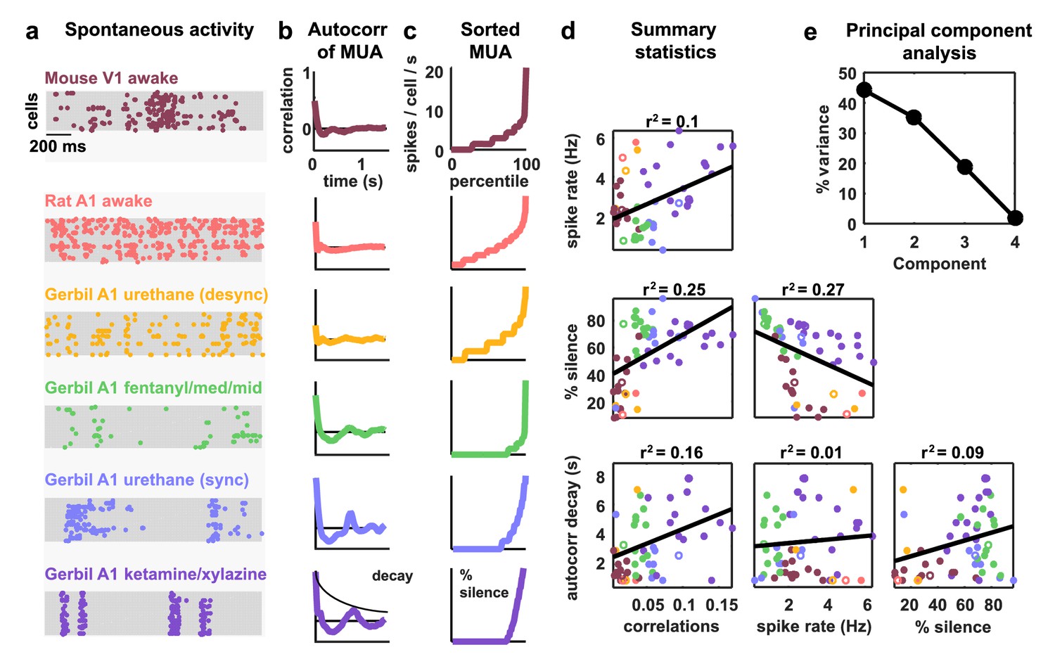
Cortical networks exhibit a wide variety of intrinsic dynamics.
(a) Multi-neuron raster plots showing examples of a short segment of spontaneous activity from each of our recording types. Each row in each plot represents the spiking of one single unit. Note that recordings made under urethane were separated into two different recording types, synchronized (sync) and desynchronized (desync), as described in the Materials and methods. (b) The autocorrelation function of the multi-unit activity (MUA, the summed spiking of all neurons in the population in 15 ms time bins) for each example recording. The timescale of the autocorrelation function (the autocorr decay) was measured by fitting an exponential function to its envelope as indicated. (c) The values of the MUA across time bins sorted in ascending order. The percentage of time bins with zero spikes (the ‘% silence’) is indicated. (d) Scatter plots showing all possible pairwise combinations of the summary statistics for each recording. Each point represents the values for one recording. Colors correspond to recording types as in (a). The recordings shown in (a) are denoted by open circles. The best fit line and the fraction of the variance that it explained are indicated on each plot. Spearman rank correlation p-values for each plot (from left to right, top to bottom) are as follows: . (e) The percent of the variance in the summary statistics across recordings that is explained by each principal component of the values.
Figure 1—figure supplement 1
Statistics for all fits.
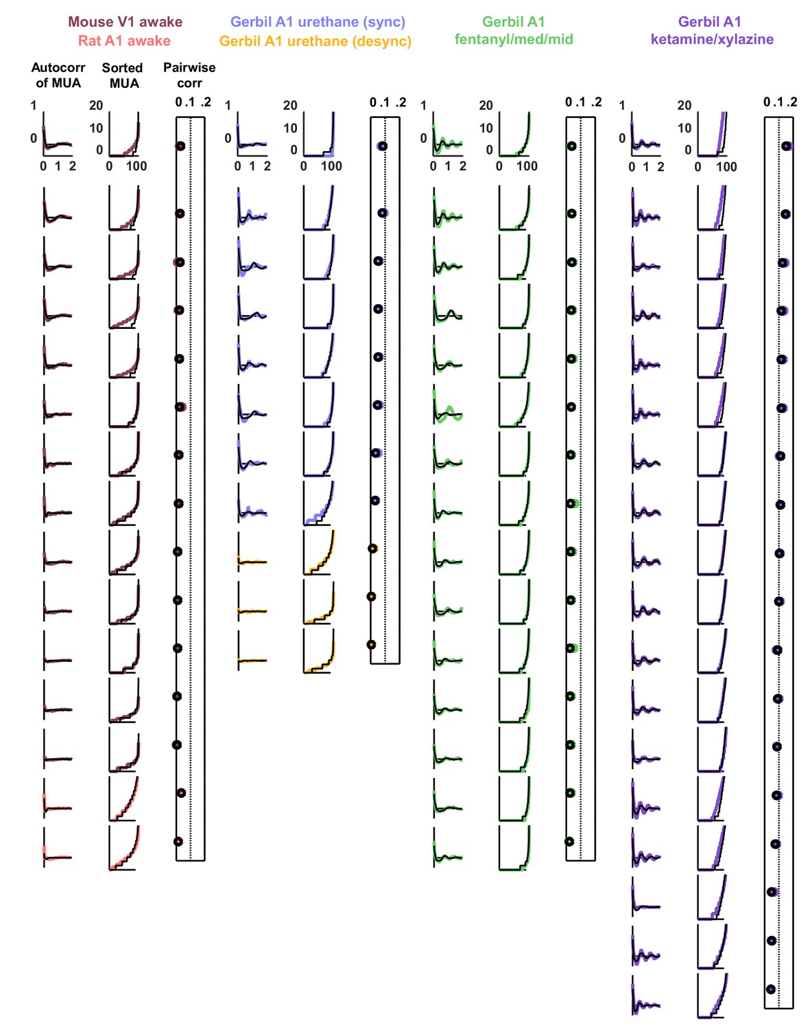
We fit the model to three statistics: (1) the autocorrelation function of the multi-unit activity (MUA, the summed spiking of all neurons in the population in 15 ms time bins), (2) the values of the MUA across time bins sorted in ascending order, and (3) the mean pairwise correlations across all pairs of neurons (in 15 ms time bins). The statistics for all 59 recordings are shown here in color. The model was fit to each of these recordings and the statistics of the activity generated by the model are shown in black.
Figure 2 with 1 supplement
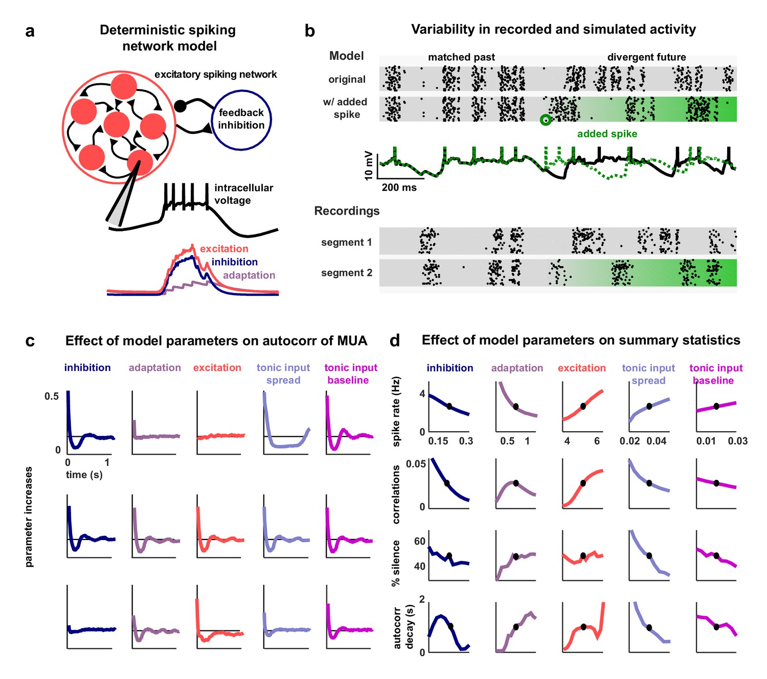
A deterministic spiking network model of cortical activity.
(a) A schematic diagram of our deterministic spiking network model. An example of a short segment of the intracellular voltage of a model neuron is also shown, along with the corresponding excitatory, inhibitory and adaptation currents. (b) An example of macroscopic variability in cortical recordings and network simulations. The top two multi-neuron raster plots show spontaneous activity generated by the model. By adding a very small perturbation, in this case one spike added to a single neuron, the subsequent activity patterns of the network can change dramatically. The middle traces show the intracellular voltage of the model neuron to which the spike was added. The bottom two raster plots show a similar phenomenon observed in vivo. Two segments of activity extracted from different periods during the same recording were similar for three seconds, but then immediately diverged. (c) The autocorrelation function of the MUA measured from network simulations with different model parameter values. Each column shows the changes in the autocorrelation function as the value of one model parameter is changed while all others are held fixed. The fixed values used were . (d) The summary statistics measured from network simulations with different model parameter values. Each line shows the changes in the indicated summary statistic as one model parameter is changed while all others are held fixed. Fixed values were as in panel c.
Figure 2—figure supplement 1
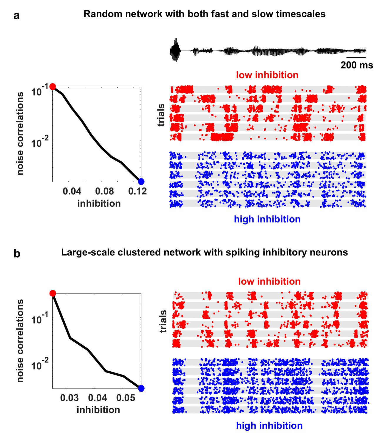
Model networks with long timescales and structured architecture.
The noise correlations are plotted as a function of the strength of feedback inhibition. Both the multi-timescale network and the clustered network produced deterministic intrinsic correlated variability in response to the IC-derived external input (as in Figure 4). This variability was quenched as inhibitory feedback was increased. The details of the networks are given in the Materials and methods.
Figure 3 with 4 supplements

Deterministic spiking networks reproduce the dynamics observed in vivo.
(a) A schematic diagram illustrating how the parameters of the network model were fit to individual multi-neuron recordings. (b) Examples of spontaneous activity from different recordings, along with spontaneous activity generated by the model fit to each recording. (c) The left column shows the autocorrelation function of the MUA for each recording, plotted as in Figure 1. The black lines show the autocorrelation function measured from spontaneous activity generated by the model fit to each recording. The middle column shows the sorted MUA for each recording along with the corresponding model fit. The right column shows the mean pairwise correlations between the spiking activity of all pairs of neurons in each recording (after binning activity in 15 ms bins). The colored circles show the correlations measured from the recordings and the black open circles show the correlations measured from spontaneous activity generated by the model fit to each recording.
Figure 3—figure supplement 1
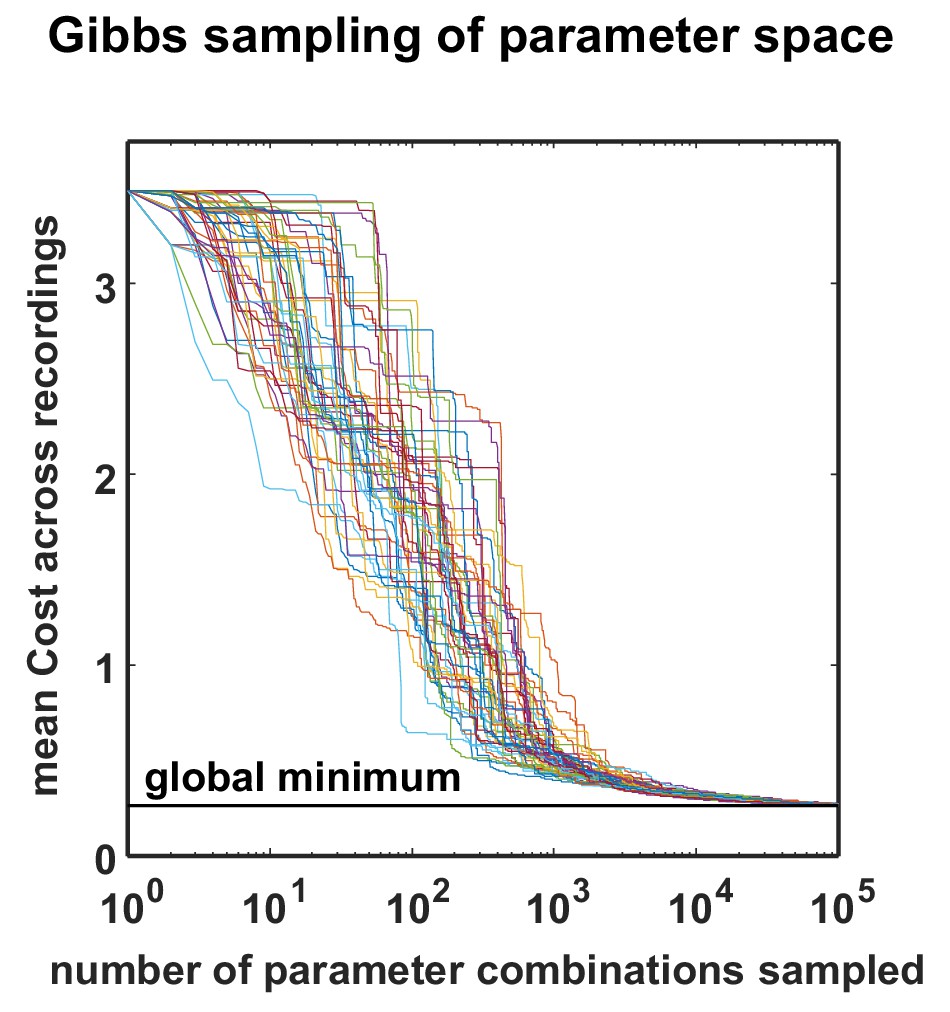
Optimization performance of the MCMC procedure.
The total cost over all recordings is plotted as a function of sample number for 50 different optimizations, started with different random seeds. All the optimizations found near-global minima for all datasets with less than 100,000 samples. To efficiently conduct this analysis, we restricted the optimizations to the already fully-sampled grid, but the optimization procedure would in general allow sampling any parameter value by using a continuous instead of a discrete proposal distribution.
Figure 3—figure supplement 2
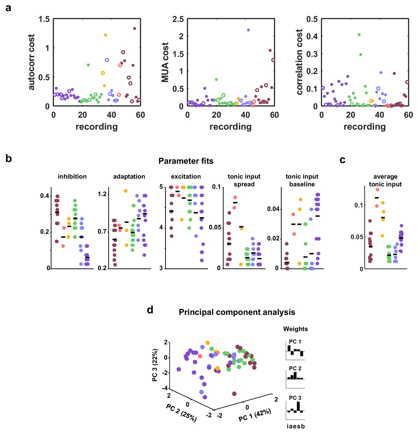
Costs and parameter fits.
(a) The three separate terms that combine into our cost function are shown for each recording. Open circles indicate datasets shown in Figure 3. (b) All parameter fits for each recording. Colors are used to indicate recordings of the same type. A small jitter was added to the horizontal location of each point. Black lines indicate median values for each recording type. (c) The average tonic input in the network fit to each recording, computed as the sum of the baseline tonic input and the mean of the exponential distribution from which the random component of the tonic input for each neuron was drawn. To compare urethane desync and urethane sync parameter values, we used a Wilcoxon rank-sum test, and found the significance of the average tonic input in desync versus sync was . The significance for adaptation, inhibition, excitation, and tonic input spread were , and , respectively. (d) A 3-dimensional principal component analysis shows that recordings generally cluster by type, but there is considerable variability both across and within recording types. The inset shows the 5-dimensional PCs.
Figure 3—figure supplement 3
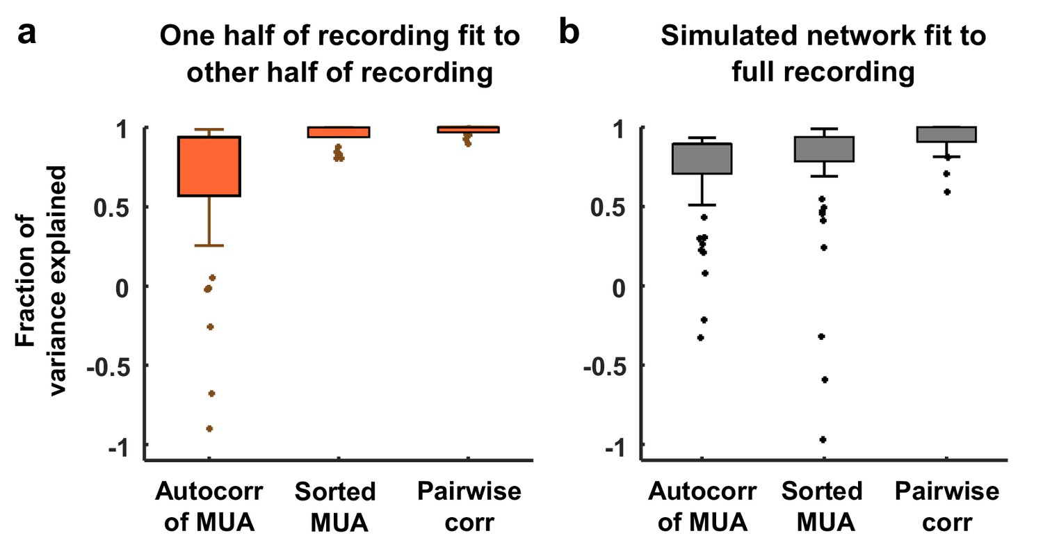
Variance explained by model fits.
(a) Each neural recording was split into two halves (interleaved segments of 4 s each) and the autocorrelation function of the MUA, the distribution of MUA values across time bins, and the mean pairwise correlations were computed for each half. The fraction of the variance in the statistics of one half of each recording that was explained by the statistics of the other half of the recording is shown. The median variance explained for the autocorrelation function of the MUA, the distribution of MUA values across time bins, and the mean pairwise correlations were 84%, 98%, and 100% respectively. (b) The amount of variance in the statistics of each full recording that was explained by the model fit is shown. The median variance explained for the autocorrelation function of the MUA, the distribution of MUA values across time bins, and the mean pairwise correlations were 82%, 90%, and 97% respectively.
Figure 3—figure supplement 4
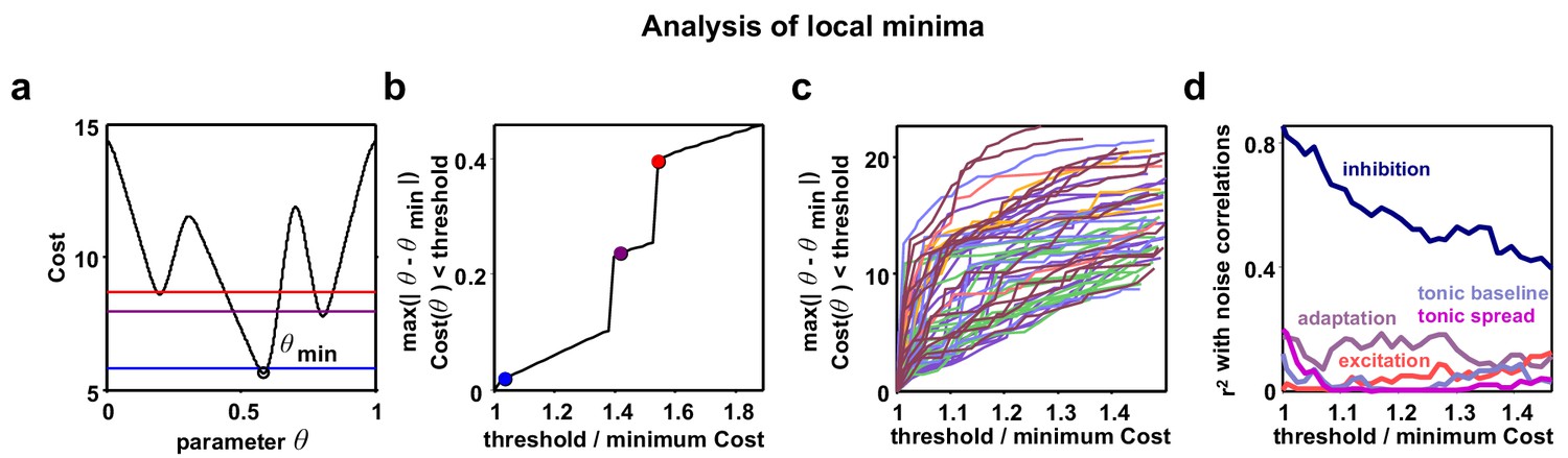
Analysis of local minima.
Parameter identifiability has recently been raised as a potential problem in interpreting the results of network simulations. To mitigate this problem, we designed our model to have a very small number of parameters and we fit three different functions of the recordings, two of which varied as a function of time or rank. To confirm that the analysis of parameter combinations other than those corresponding to the global minimum of the cost function for each recording would not lead to a different interpretation of our results, we also considered local minima in regions of parameter space that were distant from the global minimum. It is possible that such local minima correspond to parameter regimes that are qualitatively different from the global minimum, yet still capture the statistics of the recordings relatively well. We found the parameters corresponding to local minima did not consistently emphasize the role of any parameter other than inhibition; the strength of inhibitory feedback remained the dominant influence on noise correlations, even for local minima far removed from the global minimum. (a) A schematic diagram showing an example nonlinear cost function. Several different threshold values are indicated by the colored lines. All costs below threshold are considered and the parameter q furthest away from the global minimum is chosen to plot in panel b. (b) As the threshold value is increased from the global minimum, the distance of the q with Cost (q) threshold that is furthest from the global minimum is plotted. Discontinuities are visible when the threshold surpasses values at local minima. (c) Same as (b), but for the actual model fits to each recording. The values on the vertical axis are specified in terms of the grid spacing used for the Monte Carlo simulations. While some discontinuities are visible, the functions tend to increase gradually. (d) For each threshold value, we computed the between the value of each of the five model parameters and noise correlations, as in Figure 5a. This analysis shows that considering local minima situated far from the global minimum serves only to diminish the relationship between inhibition and noise correlations, without revealing any strong relationships between noise correlations and any other parameter.
Figure 4 with 1 supplement

Deterministic spiking networks reproduce the noise correlations observed in vivo.
(a) Multi-neuron raster plots and PSTHs showing examples of evoked responses from each of our recording types. Each row in each raster plot represents the spiking of one single unit. Each raster plot for each recording type shows the response on a single trial. The PSTH shows the MUA averaged across all presentations of the stimulus. Different stimuli were used for different recording types (see Materials and methods). (b) A scatter plot showing the mean spike rates and mean pairwise noise correlations (after binning the evoked responses in 15 ms bins) for each recording. Each point represents the values for one recording. Colors correspond to recording types as in (a). Values are only shown for the 38 of 59 recordings that contained both spontaneous activity and evoked responses. The Spearman's rank correlation was significant with p=0.0105. (c) A schematic diagram illustrating the modelling of evoked responses. We constructed the external input using recordings of responses from more than 500 neurons in the inferior colliculus (IC), the primary relay nucleus of the auditory midbrain that provides the main input to the thalamocortical circuit. We have shown previously that the Fano factors of the responses of IC neurons are close to one and the noise correlations between neurons are extremely weak (Garcia-Lazaro et al., 2013), suggesting that the spiking activity of a population of IC neurons can be well described by series of independent, inhomogeneous Poisson processes. To generate the responses of each model network to the external input, we averaged the activity of each IC neuron across trials, grouped the IC neurons by their preferred frequency, and selected a randomly chosen subset of 10 neurons from the same frequency group to drive each cortical neuron. (d) The top left plot shows the sound waveform presented in the IC recordings used as input to the model cortical network. The top right plot shows PSTHs formed by averaging IC responses across trials and across all IC neurons in each preferred frequency group. The raster plots show the recorded responses of two cortical populations on successive trials, along with the activity generated by the network model fit to each recording when driven by IC responses to the same sounds. (e) A scatter plot showing the noise correlations of responses measured from the actual recordings and from simulations of the network model fit to each recording when driven by IC responses to the same sounds. The Spearman rank correlation for the recordings versus the model were . The recordings shown in (d) are denoted by open circles.
Figure 4—figure supplement 1

Parameter sweeps for responses to external input.
Parameter sweeps were performed for each recording and each parameter. Each line corresponds to the model fit to one of the 59 recordings. All parameters were fixed at the values fit to each recording, except for the parameter indicated on the horizontal axis, which was swept across a wide range. Activity was generated from the model with these parameters and driven by the IC-derived external input. The spike rate, noise correlations, tuning width and percent decoding error were computed as described for Figure 5.
Figure 5
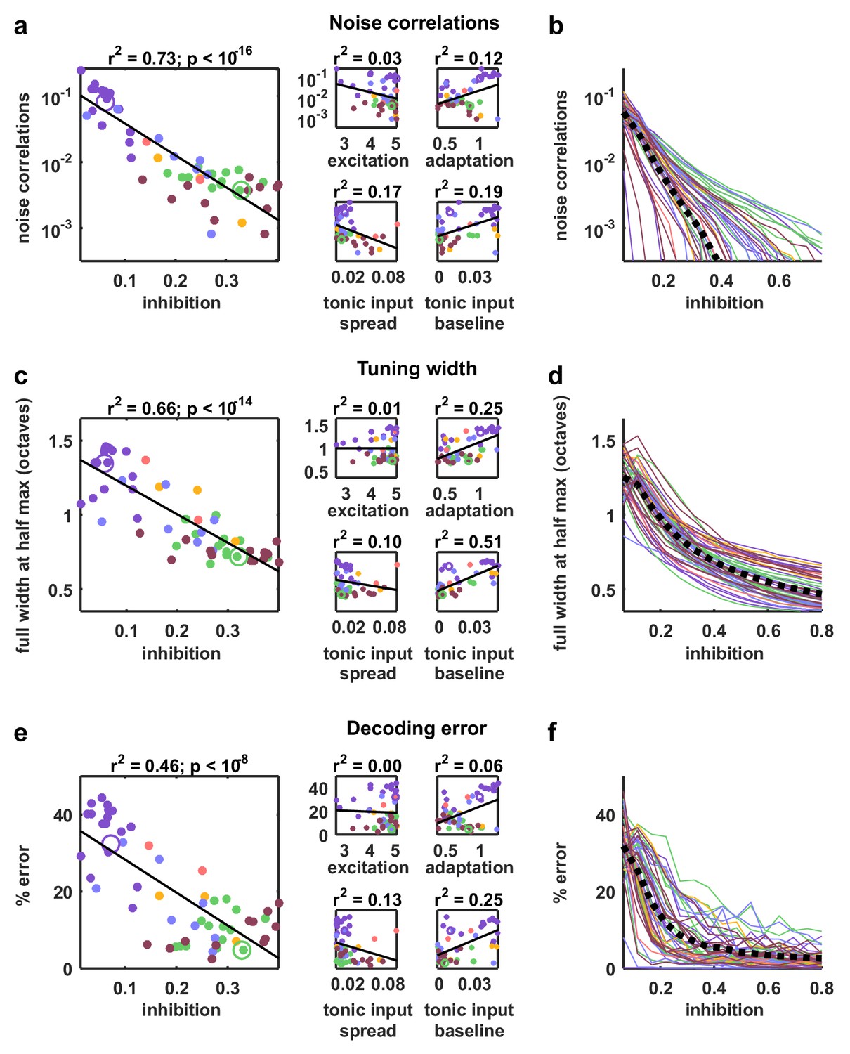
Strong inhibition suppresses noise correlations and enhances selectivity and decoding.
(a) Scatter plots showing the mean pairwise noise correlations measured from simulations of the network model fit to each recording when driven by external input versus the value of the different model parameters. Colors correspond to recording types as in Figure 4. The recordings shown in Figure 4d are denoted by open circles. Spearman's rank correlation p-values for inhibition, excitation, adaptation, tonic input spread, and tonic input baseline were , and respectively. (b) The mean pairwise noise correlations measured from network simulations with different values of the inhibition parameter . The values of all other parameters were held fixed at those fit to each recording. Each line corresponds to one recording. Colors correspond to recording types as in Figure 4. (c,e) Scatter plots showing tuning width and decoding error, plotted as in (a). For (c), Spearman rank correlation p-values for inhibition, excitation, adaptation, tonic input spread, and tonic input baseline were , and respectively. For (e), Spearman rank correlation p-values for inhibition, excitation, adaptation, tonic input spread, and tonic input baseline were , and respectively. (d,f) The tuning width and decoding error measured from network simulations with different values of the inhibition parameter , plotted as in (b).
Figure 6 with 1 supplement
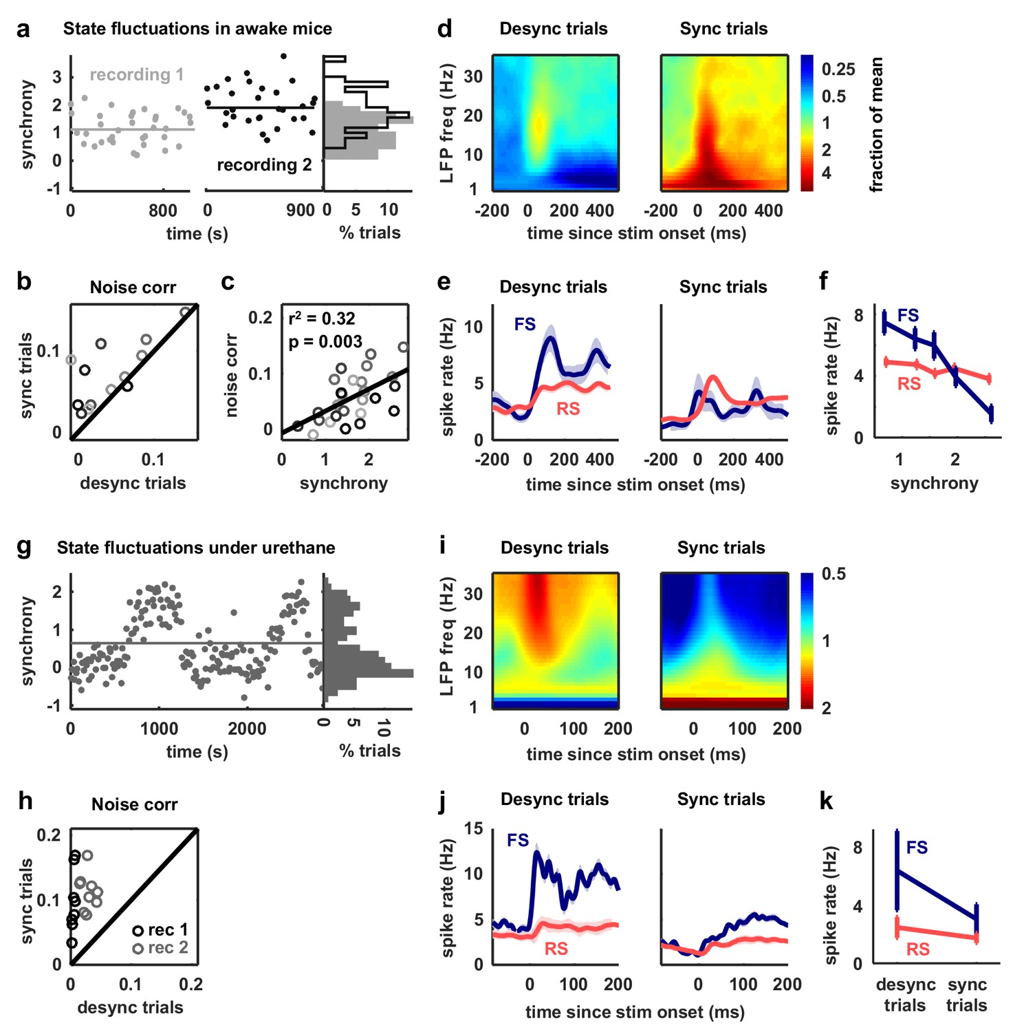
Fast-spiking neurons are more active during periods of cortical desynchronization with weak noise correlations.
(a) The cortical synchrony at different points during two recordings from V1 of awake mice, measured as the log of the ratio of low-frequency (3–10 Hz) LFP power to high-frequency (11–96 Hz). The distribution of synchrony values across each recording is also shown. The lines indicate the median of each distribution. (b) A scatter plot showing the noise correlations measured during trials in which the cortex was in either a relatively synchronized (sync) or desynchronized (desync) state for each recording. Each point indicates the mean pairwise correlations between the spiking activity of all pairs of neurons in one recording (after binning the activity in 15 ms bins). Trials with the highest 50% of synchrony values were classified as sync and trials with the lowest 50% of synchrony values were classified as desync. Values for 13 different recordings are shown. The Wilcoxon two-sided signed-rank test p-value was . (c) A scatter plot showing noise correlations versus the mean synchrony for trials with the highest and lowest 50% of synchrony values for each recording. Colors indicate different recordings. The Spearman rank correlation significance among all recordings was . (d) Spectrograms showing the average LFP power during trials with the highest (sync) and lowest (desync) 20% of synchrony values across all recordings. The values shown are the deviation from the average spectrogram computed over all trials. (e) The average PSTHs of FS and RS neurons measured from evoked responses during trials with the highest (sync) and lowest (desync) 20% of synchrony values across all recordings. The lines show the mean across all neurons, and the error bars indicate ±1 SEM. (f) The median spike rate of FS and RS neurons during the period from 0 to 500 ms following stimulus onset, averaged across trials in each synchrony quintile. The lines show the mean across all neurons, and the error bars indicate ±1 SEM. The Wilcoxon two-sided signed-rank test comparing FS activity between the highest and lowest quintile had a significance of and for RS activity, the significance was . (g) The cortical synchrony at different points during a urethane recording, plotted as in (a). The line indicates the value used to classify trials as synchronized (sync) or desynchronized (desync). (h) A scatter plot showing the noise correlations measured during trials in which the cortex was in either a synchronized (sync) or desynchronized (desync) state. Values for two different recordings are shown. Each point for each recording shows the noise correlations measured from responses to a different sound. The Wilcoxon two-sided signed-rank test between sync and desync state noise correlations had a significance of . (i) Spectrograms showing the average LFP power during synchronized and desynchronized trials, plotted as in (d). (j) The average PSTHs of FS and RS neurons during synchronized and desynchronized trials, plotted as in (e). (k) The median spike rate of FS and regular-spiking RS neurons during the period from 0 to 500 ms following stimulus onset during synchronized and desynchronized trials. The points show the mean across all neurons, and the error bars indicate ±1 SEM. The Wilcoxon two-sided signed-rank test comparing FS activity between the sync and desync had a significance of and for RS activity, the significance was .
Figure 6—figure supplement 1
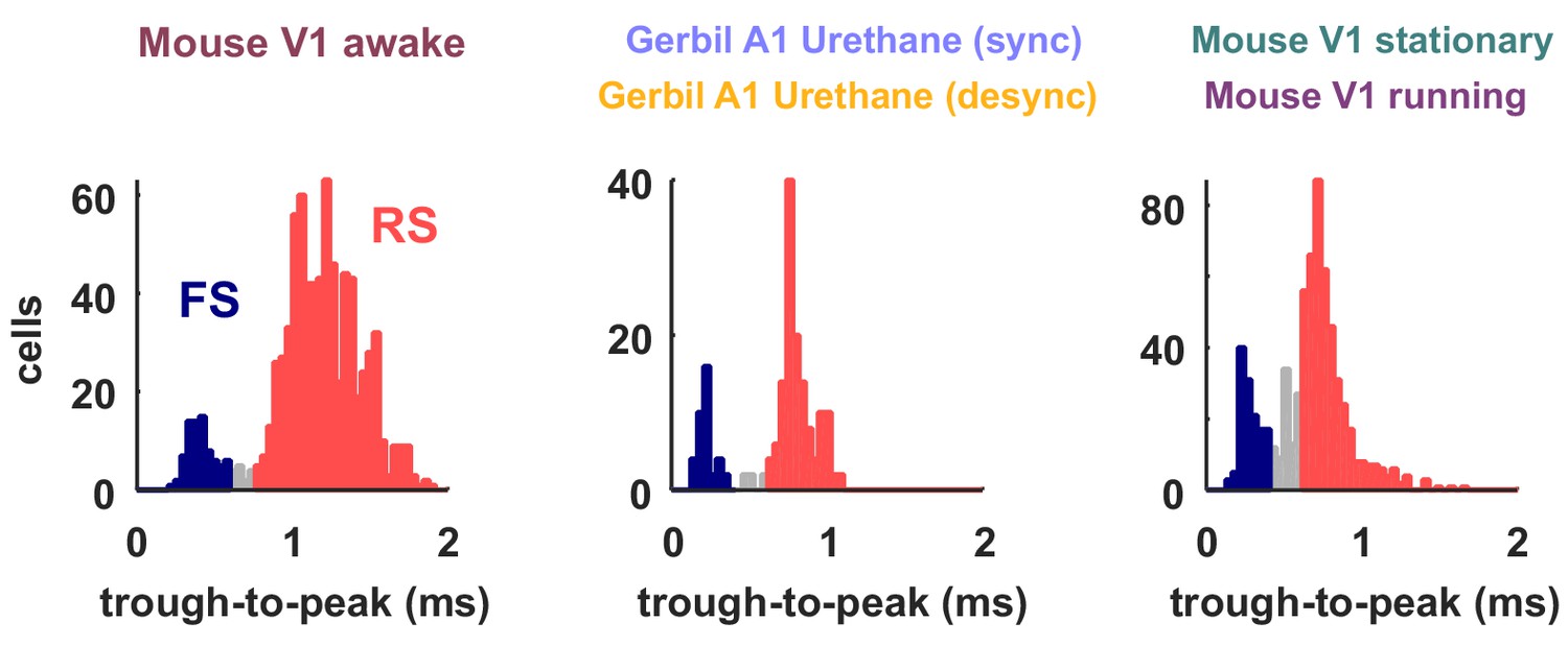
Classification of neuron types by spike width.
The spike widths of the classified spike waveforms are plotted as histograms for the different recording types. The neurons classified as FS based on their width are colored in red and the RS in blue. These were the neurons used to compute FS and RS spike rates in Figures 6 and 7. Neurons that were not clearly part of either class, which were not included in the analyses in Figures 6 and 7, are shown in gray.
Figure 7 with 1 supplement
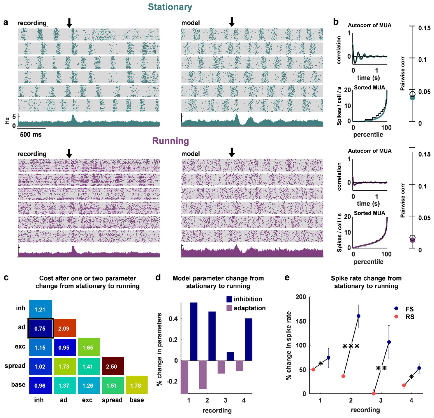
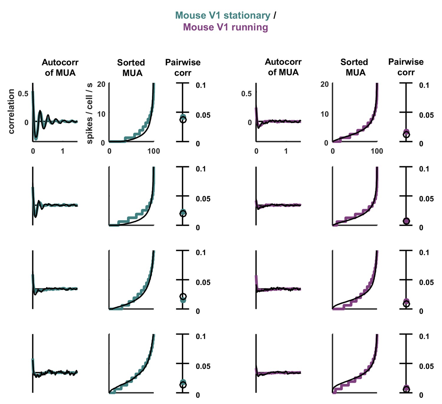
The change in dynamics during locomotion is best explained by an increase in inhibition and a reduction in adaptation.
(a) We recorded populations of neurons in head-fixed mice that were allowed to run on a treadmill. We obtained four separate recordings from two mice, which we divided into running and stationary epochs. The raster plots and PSTHs show evoked responses recorded of one example population when the animal was stationary (top) or running (bottom), along with the activity generated by the network model fit to each set of epochs. The units for the vertical axis on the PSTH are spikes / cell / s. The arrow indicates stimulus onset. (b) Model and data summary statistics for stationary (top) and running (bottom) epochs for one example population, plotted as in Figure 3. The model fits shown for running epochs were achieved by allowing two parameters (inhibition and adaptation) to change from fits to stationary epochs. (c) We fit our network model to activity from stationary epochs and investigated which changes in either one or two parameters best captured the change in dynamics that followed the transition to running. The best achieved cost with changes in each parameter (values along diagonal), or pair of parameters (values off diagonal), is shown (lower is better). (d) For the pair of parameters that best described the change in dynamics that followed the transition to running, model inhibition increased and adaptation decreased for each recording. (e) The spike rates of both FS and RS neurons were increased by running, but the relative increase was significantly larger for FS neurons in all four recordings (Wilcoxon rank-sum test, respectively). Across all recorded neurons, FS activity increased by 87% and RS activity increased by 28% during running (Wilcoxon rank-sum test, ).
Figure 7—figure supplement 1
Statistics for all fits.
The model was fit to stationary and running epochs for each of four separate recordings. The statistics of the activity measured from the recordings and generated by the model fit to the recordings are shown, plotted as in Figure 3.
Additional files
-
Supplementary file 1
Metadata for all recordings.
The table shows the species, brain region, and state for each of our recordings, as well information regarding the stimuli presented and the number of neurons recorded.
- https://doi.org/10.7554/eLife.19695.019
-
Supplementary file 2
Species and brain area for studies of cortical dynamics cited in the Discussion.
The table shows the species and brain region for the studies cited in the sections of the Discussion related to cortical dynamics.
- https://doi.org/10.7554/eLife.19695.020
Download links
A two-part list of links to download the article, or parts of the article, in various formats.
Downloads (link to download the article as PDF)
Open citations (links to open the citations from this article in various online reference manager services)
Cite this article (links to download the citations from this article in formats compatible with various reference manager tools)
Inhibitory control of correlated intrinsic variability in cortical networks
eLife 5:e19695.
https://doi.org/10.7554/eLife.19695


