Transcription leads to pervasive replisome instability in bacteria
- University of Washington, United States
Figures
Figure 1 with 6 supplements
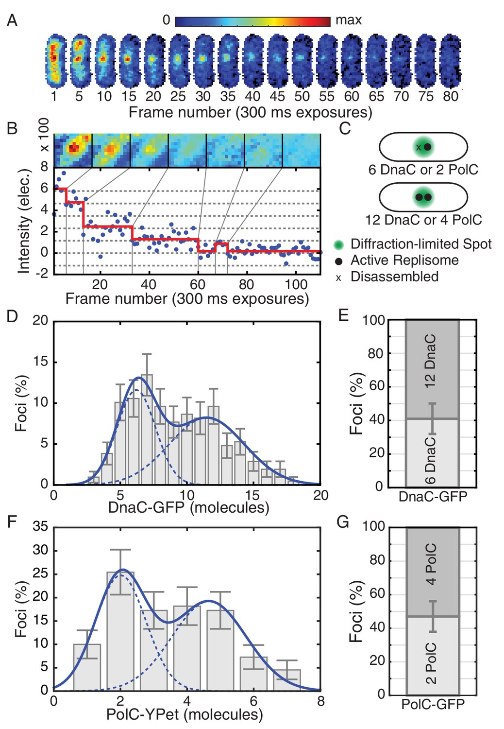
Estimated stoichiometry distributions for core replisome proteins in B. subtilis.
(A) Photobleaching of DnaC-GFP in a replication factory. (B) A typical intensity trace (blue) is shown for a DnaC-GFP focus. Stepwise transitions are observed as the fluorescent protein bleaches. The intensity is filtered using Change-Point analysis (red) which determines the intensity step-size corresponding to the bleaching of single fluorophores (complete stoichiometry calculation is demonstrated in Figure 1—figure supplements 2 and 3, and detailed in the materials and methods section). The image mosaic above shows the time-averaged image of the focus over each intensity level. (C) A schematic of the replication factory consisting of either one or two assembled replisomes (black dots) in a diffraction-limited spot (green). (D) Histogram of estimated factory DnaC-GFP stoichiometry in B. subtilis. Error bars represent counting error. The observed distribution is well fit by a two Gaussian model (solid blue), representing a mixed population of single-helicase (6 DnaC molecules) and two-helicase (12 DnaC molecules) factories. (Analysis for N = 213 factories.) (E) Relative abundance of factories with one and two helicases. (F) Estimated stoichiometry distribution for PolC-YPet in B. subtilis shows two populations (N = 125). Peak stoichiometries for each population (dashed blue) were determined by maximum likelihood fitting with a two Gaussian model (solid blue) to be 2 and 4 copies. (Note: the distribution included a small fraction (~5%) of factories with stoichiometries greater than 10 copies which were removed for the purpose of fitting.) (G) Relative abundance of factories with 2 and 4 copies of PolC-GFP.
Figure 1—figure supplement 1
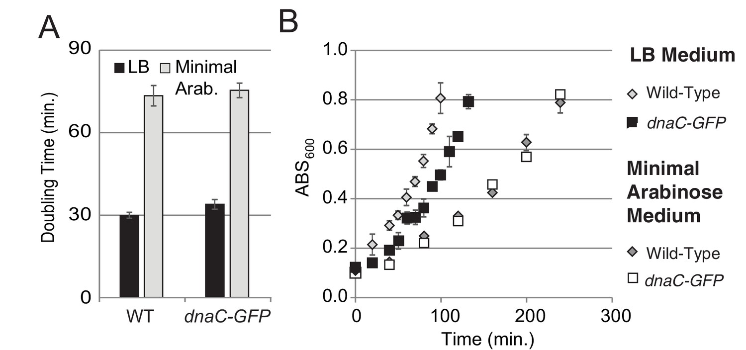
Growth curves for DnaC-GFP.
For growth curves, the optical density of wild type and dnaC-gfp strains growing in minimal arabinose medium at 30°C were monitored for 5 hr. Linear regression to OD600 readings were used to determine doubling time. (A) The dnaC-gfp allele does not confer a detectable growth defect in minimal medium. OD600 readings for a representative culture of wild type and dnaC-gfp cells. (B) Calculated doubling times and OD600 readings show a small growth defect for the dnaC-gfp strain relative to wild type in LB medium.
Figure 1—figure supplement 2
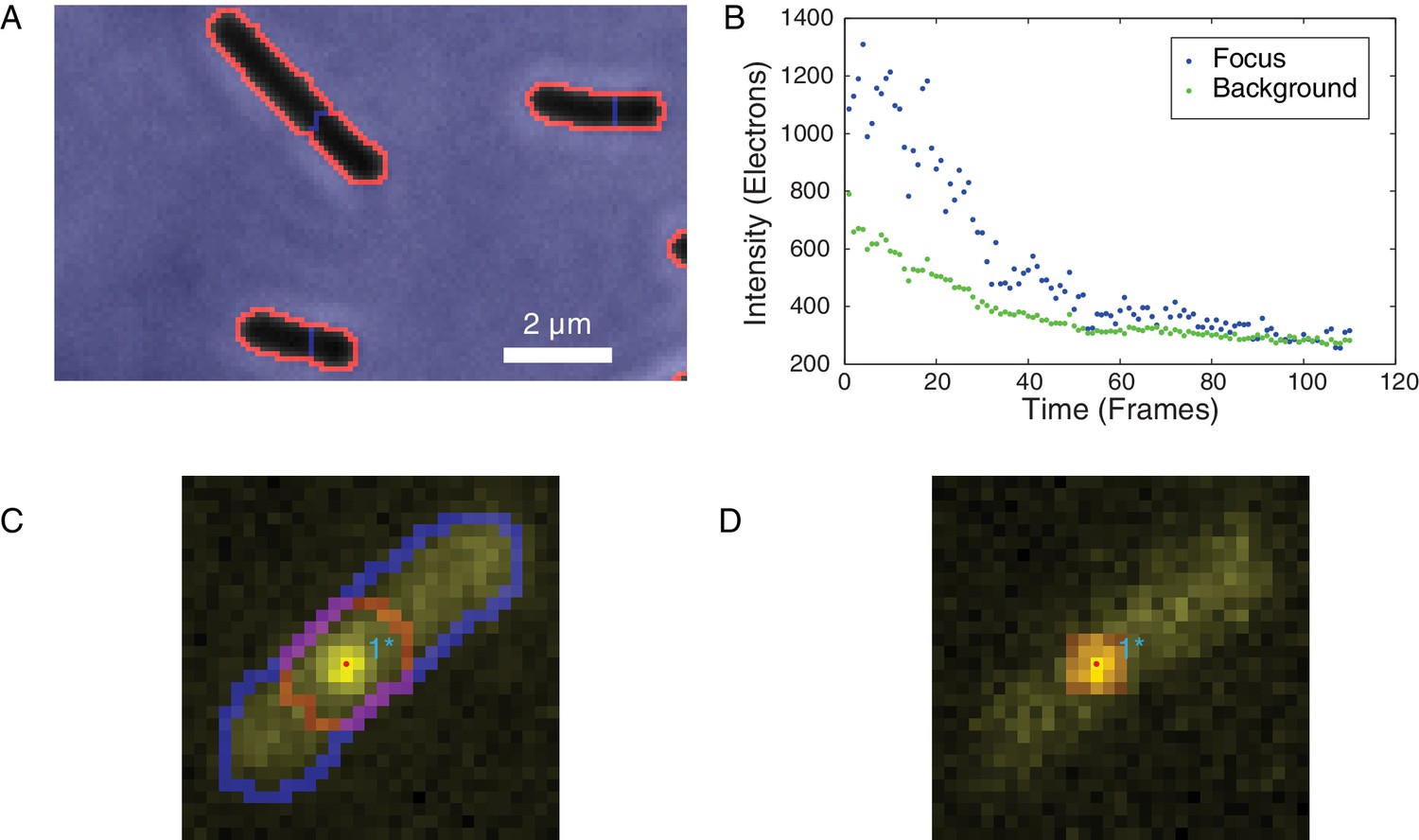
Identification of foci and determination of raw focus intensity.
(A) The phase-contrast image of the cells was segmented to identify the cell boundaries (orange) surrounding each cell mask (black). (B) The integrated raw focus intensity (blue) and scaled background intensity (green) are plotted for a bleaching experiment. The intensity trace is computed by subtracting the background from the raw intensity. (C) The summed image is shown in yellow. The outline of the cell mask is shown in blue. The intensity regions (red outline) are determined by watersheding the summed intensity to divide the image into local maxima. The focus positions (points) are determined by fitting a Gaussian distribution in the intensity regions. (D) The raw focus intensity is determined by summing the intensity in a mask centered on the locus position. The background is computed by calculating the average intensity inside the cell (blue outline) but outside the intensity region (red).
Figure 1—figure supplement 3
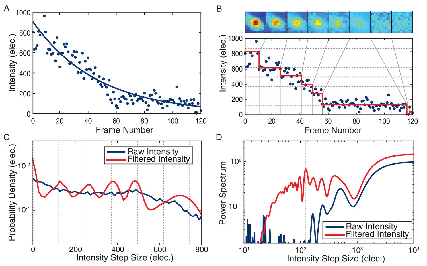
Stoichiometry calculation demonstrated for a DnaC-GFP focus.
(A) Intensity tracking of a DnaC-GFP focus in B. subtilis. A decaying exponential (solid blue) is fit to the background subtracted raw intensities (blue points) traced over a series of 120 fluorescence images. The value of the exponential fit in the first frame is taken as the initial intensity of the DnaC-GFP complex (see methods). (B) The raw intensities (solid blue) are filtered (mean value in red) to reveal stepwise transitions. Summed fluorescence images of the DnaC-GFP complex are shown corresponding to each level detected by the filter in the image strip above the plot area. (C) The PPDD of the filtered intensities (red) reveals peaks at integral multiples of the unitary intensity step that would not be detectable in PPDD of the raw intensities (blue). (D) The power spectrum is used to identify the location of the first order peak in the PPDD which corresponds to the highest peak in the power spectrum (dashed gray). The unitary intensity step determined by the power spectrum corresponds to the spacing of the dashed gray lines in panels B and C.
Figure 1—figure supplement 4
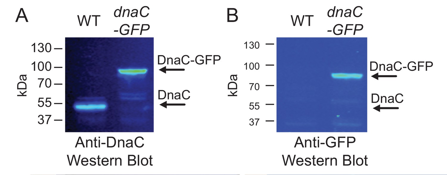
Western blots for DnaC-GFP.
Cells produce complete DnaC-GFP fusion protein. Western blot analysis indicates that DnaC-GFP is fully synthesized, and that potentially truncated DnaC proteins lacking GFP are not detected. Individual lanes were normalized by total protein, and separate western blots were probed with either (A) anti-DnaC polyclonal antibodies or (B) anti-GFP polyclonal antibodies.
Figure 1—figure supplement 5
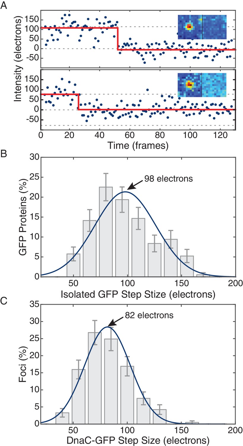
Comparison of in vivo and in vitro step sizes for GFP.
(A) Bleaching traces for two different surface immobilized GFP proteins. Inserts show the mean fluorescence images in the bleached and unbleached states. (B) Maximum likelihood fits to unitary intensity step distributions for isolated GFP in vitro. (C) Example in vivo unitary step distribution for DnaC-GFP in B. subtilis and its maximum likelihood fit. For all experimental conditions in B. subtilis, unitary step distributions were peaked within 19% found in vitro value.
Figure 1—figure supplement 6
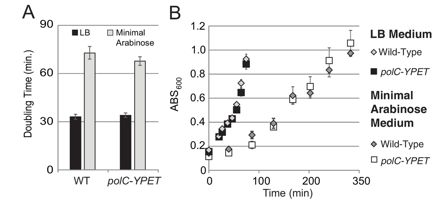
Growth curves for PolC-YPet.
For growth curves, the optical density of wild type and polC-YPET strains growing in minimal arabinose medium at 30°C were monitored for 5 hr. Linear regression to OD600 readings were used to determine doubling time. (A–B) No growth defect is observed for polC-ypet in either minimal or LB growth medium.
Figure 2 with 3 supplements
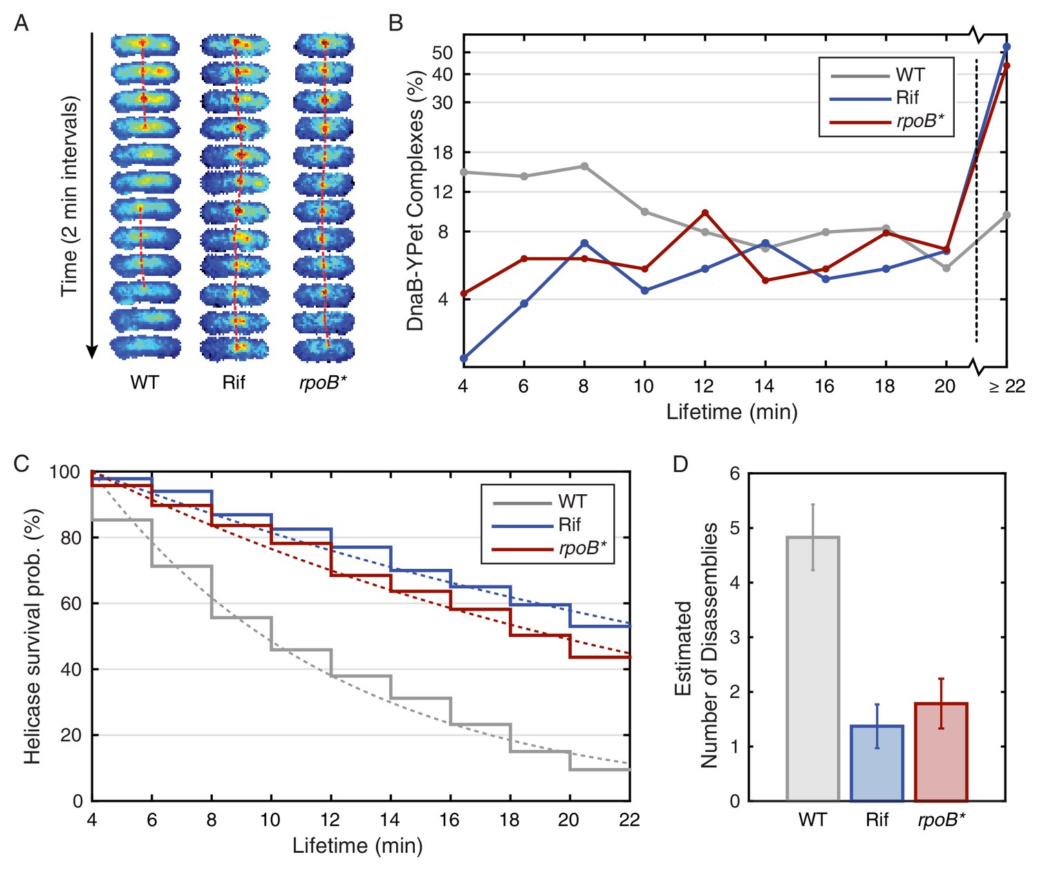
Helicase complex dynamics in B. subtilis captured by time-lapse imaging.
(A) Typical frame mosaics for dynamics of the helicase in three conditions: Untreated (WT), rifampicin-treated (Rif) and rpoB* cells (see also Figure 2—figure supplement 1). (In this context, WT refers to cells carrying the dnaC-gfp allele but not the rpoB* allele.) The helicase complexes in WT cells were observed to be intermittent: assembling and disassembling on the timescale of minutes. The helicase complexes in rifampicin-treated and rpoB* cells were observed to be more persistent. The complexes were tracked by an automated algorithm (red, detailed description in material and methods). (B) Distribution of helicase complex lifetime in WT (gray, N = 327 complexes), rifampicin-treated (blue, N = 183 complexes) and rpoB* (red, N = 165 complexes) cells. Data collection is limited to 22 min. (C) Probability of helicase survival as a function of helicase complex lifetime. Solid lines represent the empirical survival curves. Dashed lines show fits determined by maximum likelihood estimation. (D) Estimated number of disassembly events per 40 min of replication using the Poisson process model (see also Table 1). Error bars were generated by simulating 100,000 distributions with the same rate parameter and number of complexes as the observed distribution. Simulated distributions were then fit, and the width of the rate parameter distribution was used to quantify the error.
-
Figure 2—source data 1
B. subtilis lifetimes.
- https://doi.org/10.7554/eLife.19848.010
Figure 2—figure supplement 1
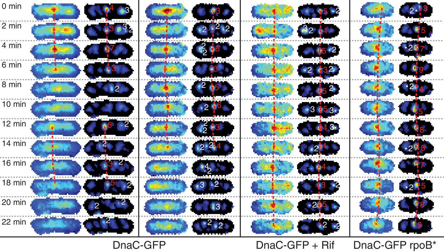
Automatic tracking of helicase complexes using focus scoring.
Under normal growth conditions, a typical trajectory resulting from dynamics analysis shows rapid appearance and disappearance of DnaC-GFP foci. Both rifampicin treatment and a rpoB* mutation results in longer-lived foci. Image strips to the left show raw images with dashed red lines indicating automatically detected trajectories. Corresponding filtered images to the right additionally show focus scores for all automatically detected foci. Scores printed in red indicate that the focus is included in a trajectory. Low scoring foci not selected for a trajectory are indicated in white. A detailed description of scoring and automated focus tracking is included in the materials and methods section.
Figure 2—figure supplement 2
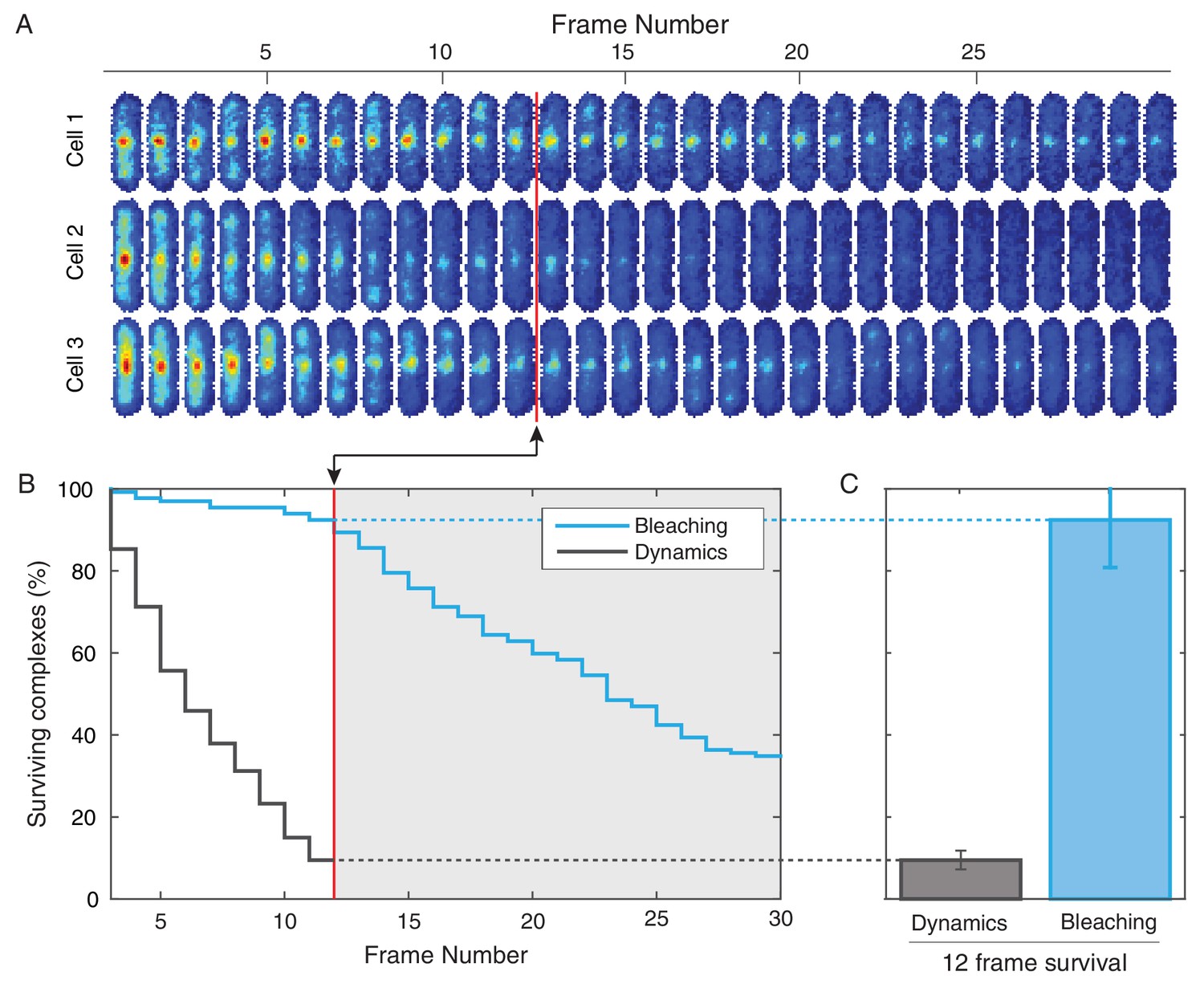
Photobleaching minimally affects the complex lifetime experiments in B. subtilis.
(A) To isolate the effects of photobleaching, cells are imaged with the same intensity and exposure as in the dynamics measurement, but with no delay between frames. Red line indicates equivalent of the 12 frame time course used in the dynamics measurement for B. subtilis. (B) Automated tracking used for the dynamics measurement was applied to the bleaching data. Survival curve (blue) shows the fraction of (N = 132) complexes that were successfully tracked through a given number of frames. Survival curve for dynamics experiment (gray) is shown for comparison. (C) 92% of complexes were traceable for 12 frames. In contrast, only 9% of complexes survive the duration of the dynamics experiment.
Figure 2—figure supplement 3
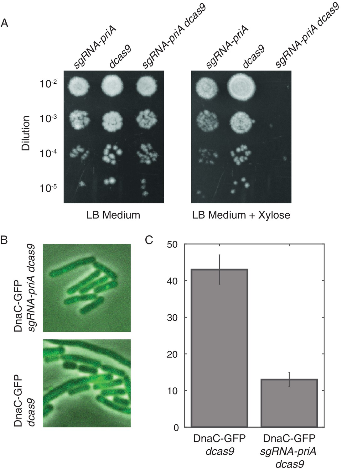
Disruption of PriA leads to loss of DnaC-GFP foci.
(A) Survival assays show that the depletion of PriA is lethal on LB medium, but the control strains (which contain either the sgRNA-priA or dcas9) survive under both conditions. We find the same result using minimal arabinose medium. (B) Sample snapshots showing the full PriA CRISPR strain, and the control (no sgRNA), both after induction with 1% xylose for approximately two hours. (C) Disruption of PriA results in a decrease in the number of cells with DnaC-GFP foci from 43% in the control strain (N = 518 cells) to 13% in the CRISPR strain (N = 413 cells). Error bars represent counting error.
Figure 3 with 3 supplements
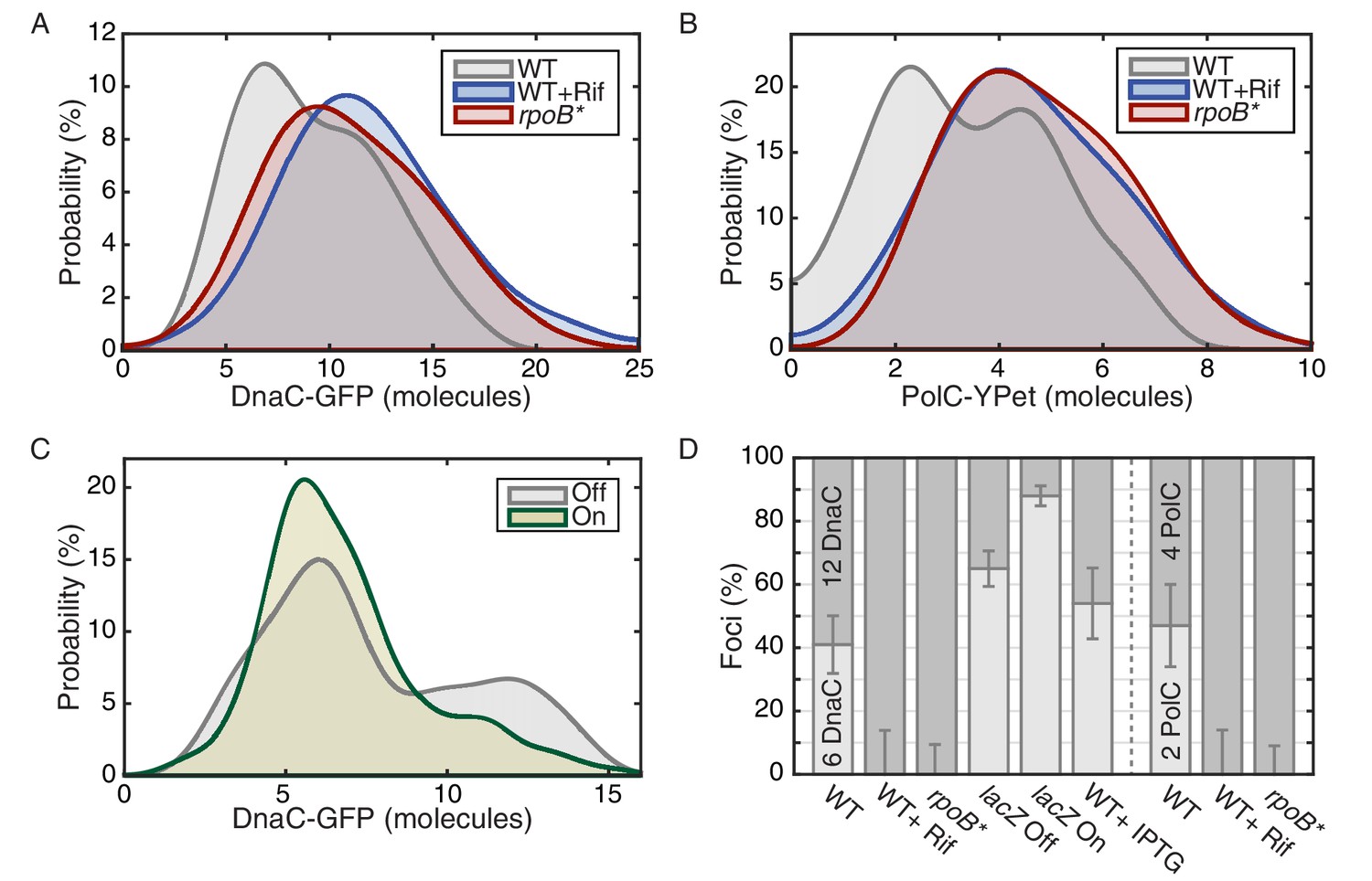
The effect of perturbations to transcription on stoichiometry distributions.
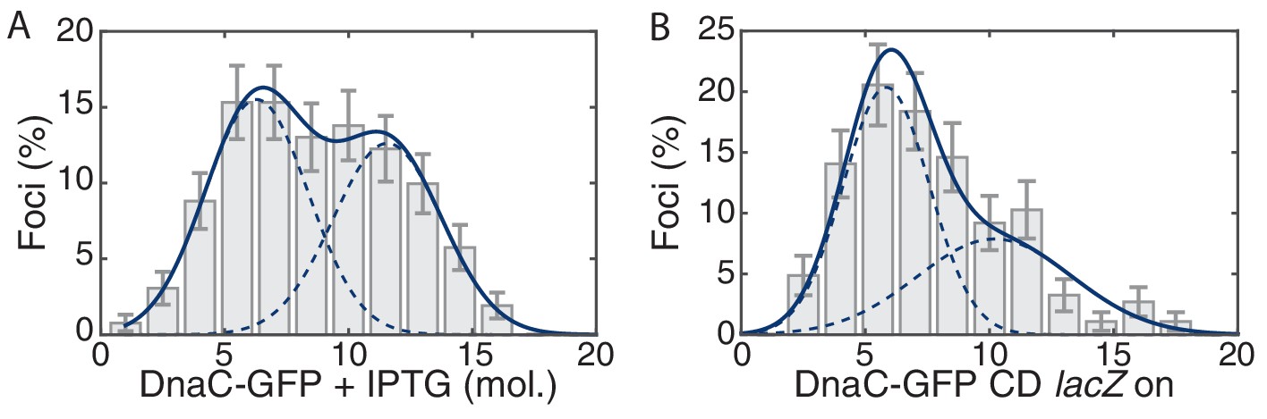
(A) Helicase complex stoichiometry under three conditions: Untreated (WT), rifampicin-treated (Rif) and rpoB* cells. Probability densities are represented as Kernel Density Estimates (KDEs). In contrast to WT (gray), in both rifampicin-treated (blue) and rpoB* (red) cells, a significant fraction of single-helicase complexes (6 DnaC molecules) are lost with all observations being consistent with two-helicase complexes (12 DnaC molecules). (N = 70–117) (B) Estimated PolC stoichiometry in untreated (gray), rifampicin-treated (blue), and rpoB* (red) cells (N = 81–125). The low stoichiometry peak is no longer resolvable after rifampicin treatment or in the rpoB* mutant background, implying increased stability of the polymerase. (Note: rifampicin treatment also increased the exceedingly high fluorescence population which was again removed for the purpose of fitting.) (C) The relative abundance of helicase complex stoichiometries in cells with an ectopic inducible head-on replication-transcription conflict (lacZ). An IPTG (induction)-dependent increase in the single-helicase stoichiometry was observed, consistent with the reduction in factory stoichiometry being conflict-induced. (N = 108–174) (D) Summary of stoichiometry for transcription-inhibition and ectopic-conflict experiments. Estimates for the relative abundance of first and second order stoichiometry sub-populations are determined by fitting the distributions of estimated stoichiometries (Figure 3—figure supplement 1, Table 2).
Figure 3—figure supplement 1
Control for head-on conflict experiment.
(A) The observed stoichiometry of DnaC-GFP was not significantly altered by the addition of IPTG. Compare to Figure 1D. (B) Addition of lacZ (transcription on) in the co-directional orientation causes a small decrease to replisome stability.
Figure 3—figure supplement 2
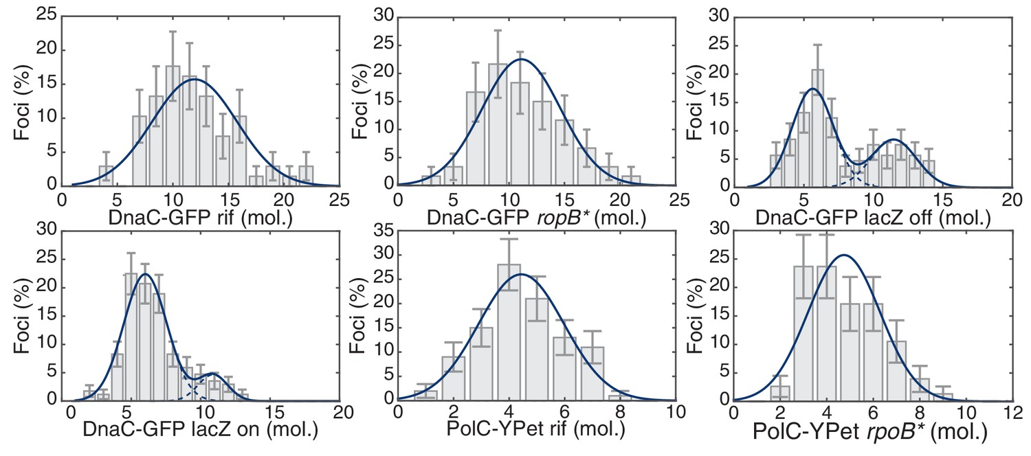
Maximum likelihood fits to B. subtilis stoichiometry distributions.
The most likely two Gaussian model is selected varying the Gaussian means, widths and peak intensities. Maximum likelihood models (blue) and comprising Gaussians (dashed blue) are shown over histogram distributions. Error bars represent counting error. Calculated maximum likelihood fit parameters are summarized in Table 2.
Figure 3—figure supplement 3
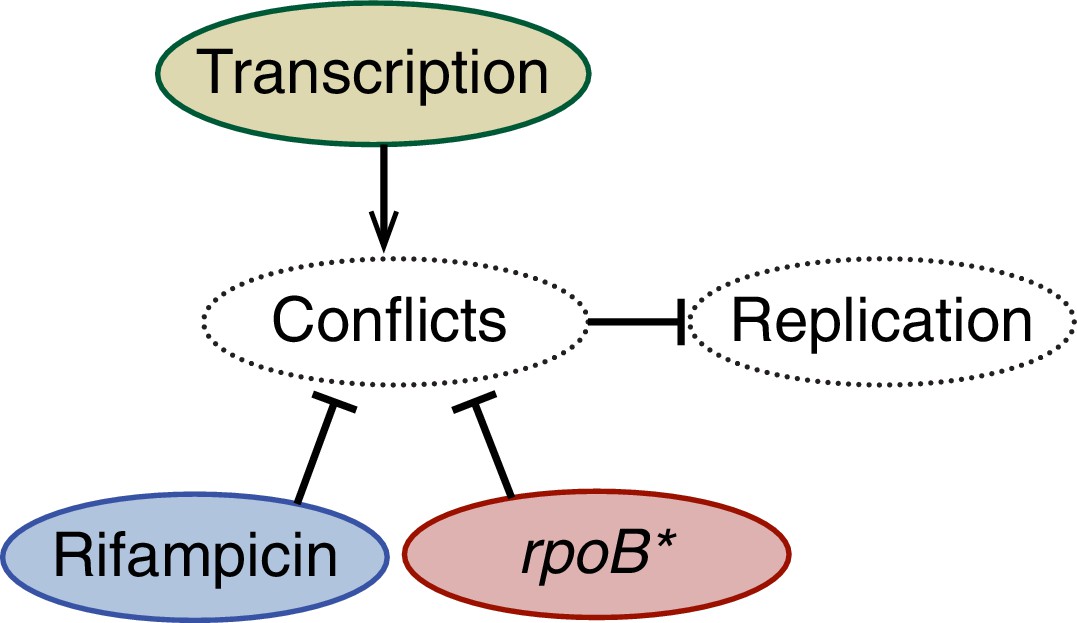
A schematic model illustrating the effects of perturbations to transcription on replisome stability.
Amelioration of conflicts both by rifampicin or an rpoB* mutant increases the stability of the replisome. Conversely, addition of a highly transcribed gene in the head-on orientation decreases replisome stability.
Figure 4 with 2 supplements
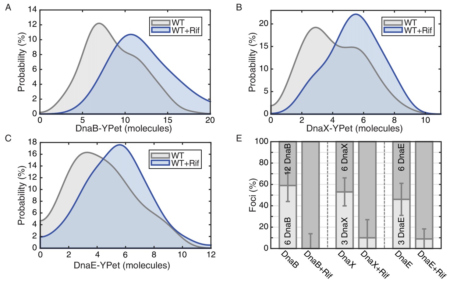
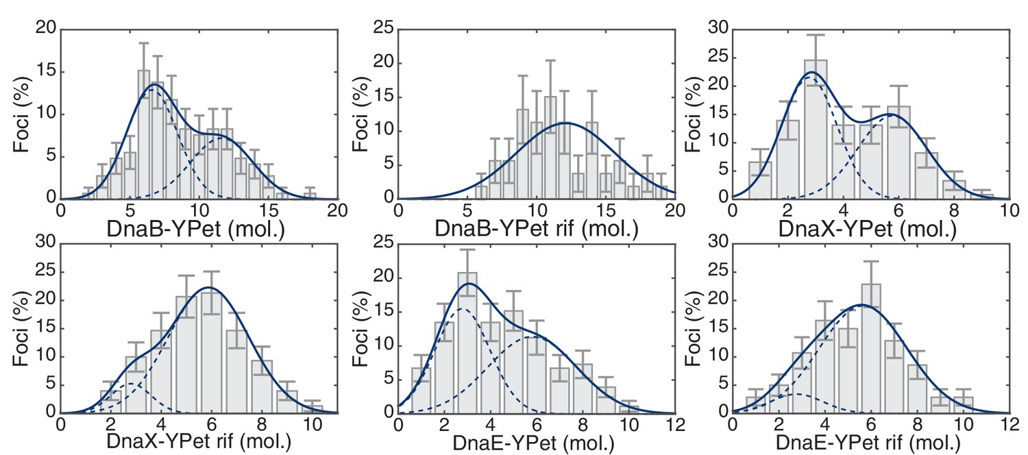
E. coli stoichiometry distributions shift similarly to those in B. subtilis under transcription inhibition.
Stoichiometry distributions are represented using kernel density estimation (N = 53–178 factories). (A) Estimated DnaB stoichiometry suggests that two hexameric helicases are present in most replication factories in the absence of transcription (blue). However, under normal conditions (gray) roughly half of factories consist of only a single helicase. (B) Transcription-inhibition increases the number of factories having higher DnaX stoichiometry. (C) Transcription-inhibition increases the number of factories having higher DnaE stoichiometry. (D) Estimates for the relative abundance of first and second order stoichiometry sub-populations are determined by fitting the distributions of estimated stoichiometries (Figure 4—figure supplement 1 and Table 3).
Figure 4—figure supplement 1
Maximum likelihood fits to E. coli stoichiometry distributions.
The most likely two Gaussian model is selected varying the Gaussian means, widths and peak intensities. Maximum likelihood models (blue) and comprising Gaussians (dashed blue) are shown over histogram distributions. Error bars represent counting error. Error bars represent counting error. Calculated maximum likelihood fit parameters are summarized in Table 3.
Figure 4—figure supplement 2
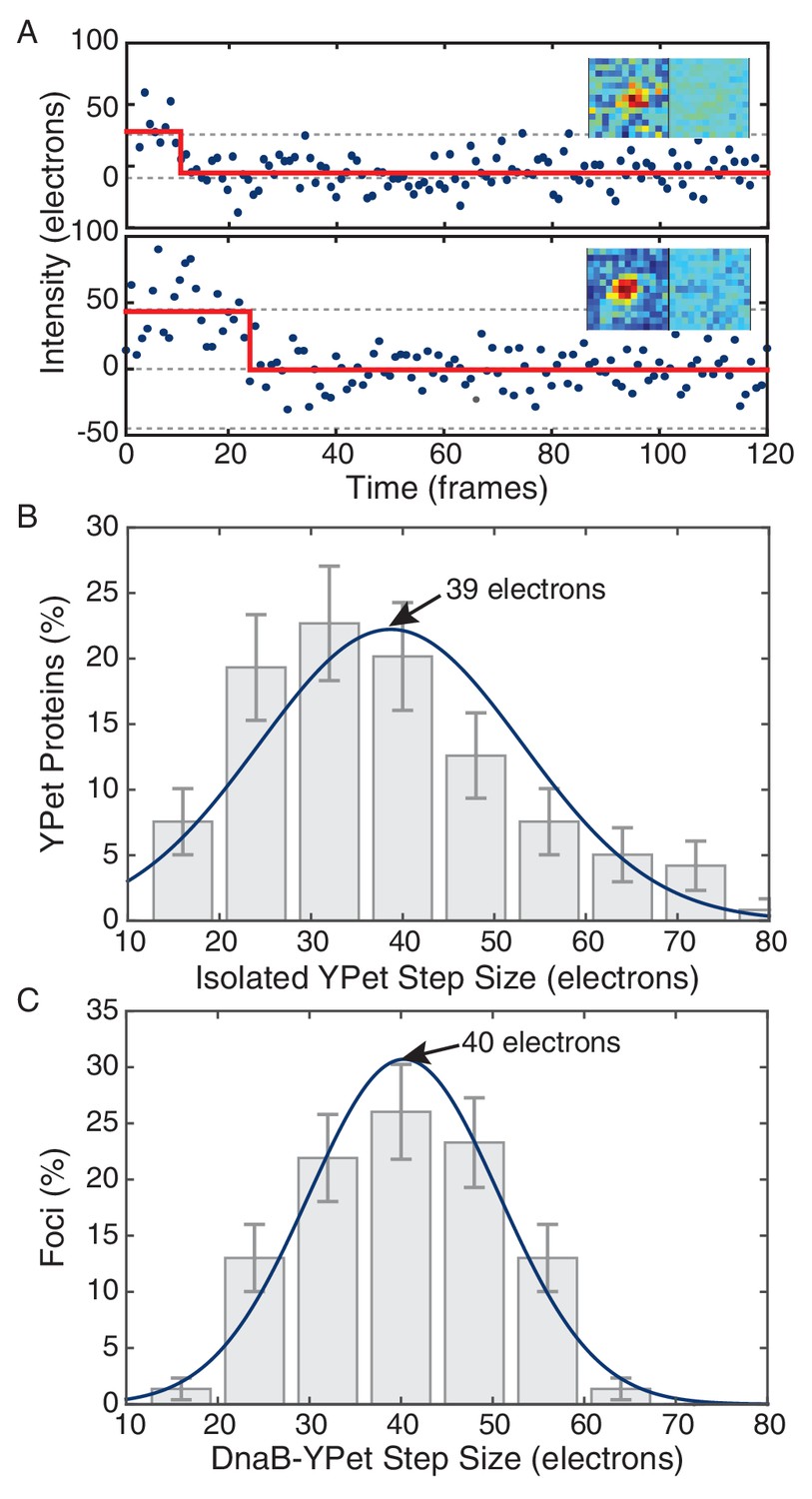
Comparison of in vivo and in vitro step sizes for YPet.
(A) Bleaching traces for two different surface immobilized YPet proteins. Inserts show the mean fluorescence images in the bleached and unbleached states. (B) Maximum likelihood fits to unitary intensity step distributions for isolated YPet in vitro. (C) Example in vivo unitary step distribution for DnaB-YPet in E. coli and its maximum likelihood fit. For all experimental conditions in E. coli, unitary step distributions were peaked within 18% found in vitro value.
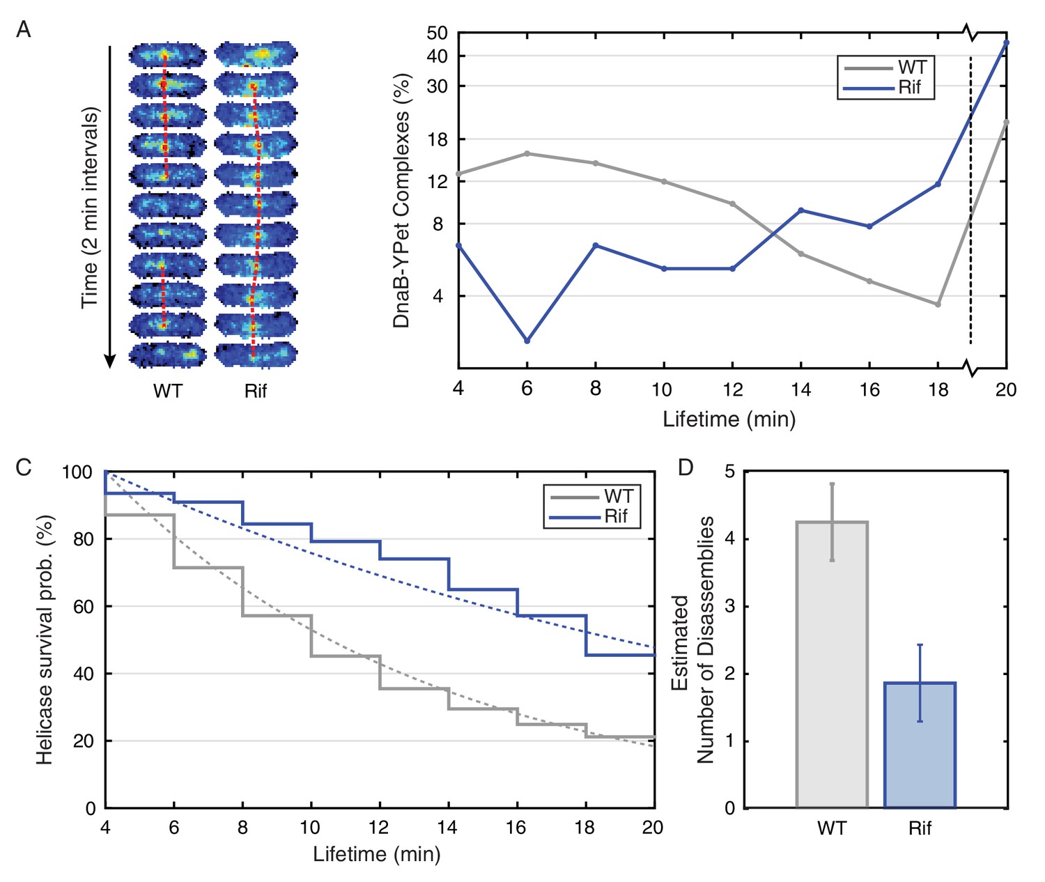
Figure 5 with 2 supplements
Helicase complex dynamics in E. coli captured by time-lapse imaging.
Helicase complex dynamics in E. coli captured by time-lapse imaging. (A) Typical frame mosaics for dynamics of the helicase in two conditions: Untreated (WT), rifampicin-treated (Rif). The helicase complexes in WT cells were observed to be intermittent: assembling and disassembling on the timescale of minutes. The helicase complexes in rifampicin-treated cells were observed to be more persistent. The complexes were tracked by an automated algorithm (red). (B) Distribution of helicase complex lifetime in WT (gray, N = 217 complexes), rifampicin-treated (blue, N = 77 complexes). Data collection is limited to 20 min. (C) Probability of helicase survival as a function of helicase complex lifetime. Solid lines represent the empirical survival curves. Dashed lines show fits determined by maximum likelihood estimation. (D) Estimated number of disassembly events per cell cycle using the Poisson process model (see also Table 4). Simulating 100,000 distributions with the same rate parameter and number of complexes as the observed distribution generated error bars. Simulated distributions were then fit, and the width of the rate parameter distribution was used to quantify the error.
-
Figure 5—source data 1
E. coli lifetimes.
- https://doi.org/10.7554/eLife.19848.025
Figure 5—figure supplement 1
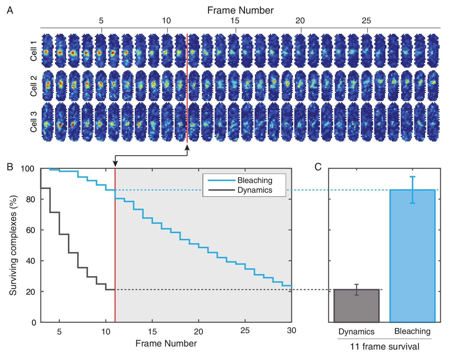
Photobleaching minimally affects the complex lifetime experiments in E. coli.
(A) To isolate the effects of photobleaching, cells are imaged with the same intensity and exposure as in the dynamics measurement, but with no delay between frames. Red line indicates equivalent of the 11 frame time course used in the dynamics measurement. (B) Automated tracking used for the dynamics measurement was applied to the bleaching data. Survival curve (blue) shows the fraction of complexes that were successfully tracked through a given number of frames (N = 214). Survival curve for the dynamics experiment (gray) is shown for comparison (C) 86% of complexes were traceable for 11 frames. In the dynamics measurement, only 21% of complexes survive the duration of the experiment.
Figure 5—figure supplement 2
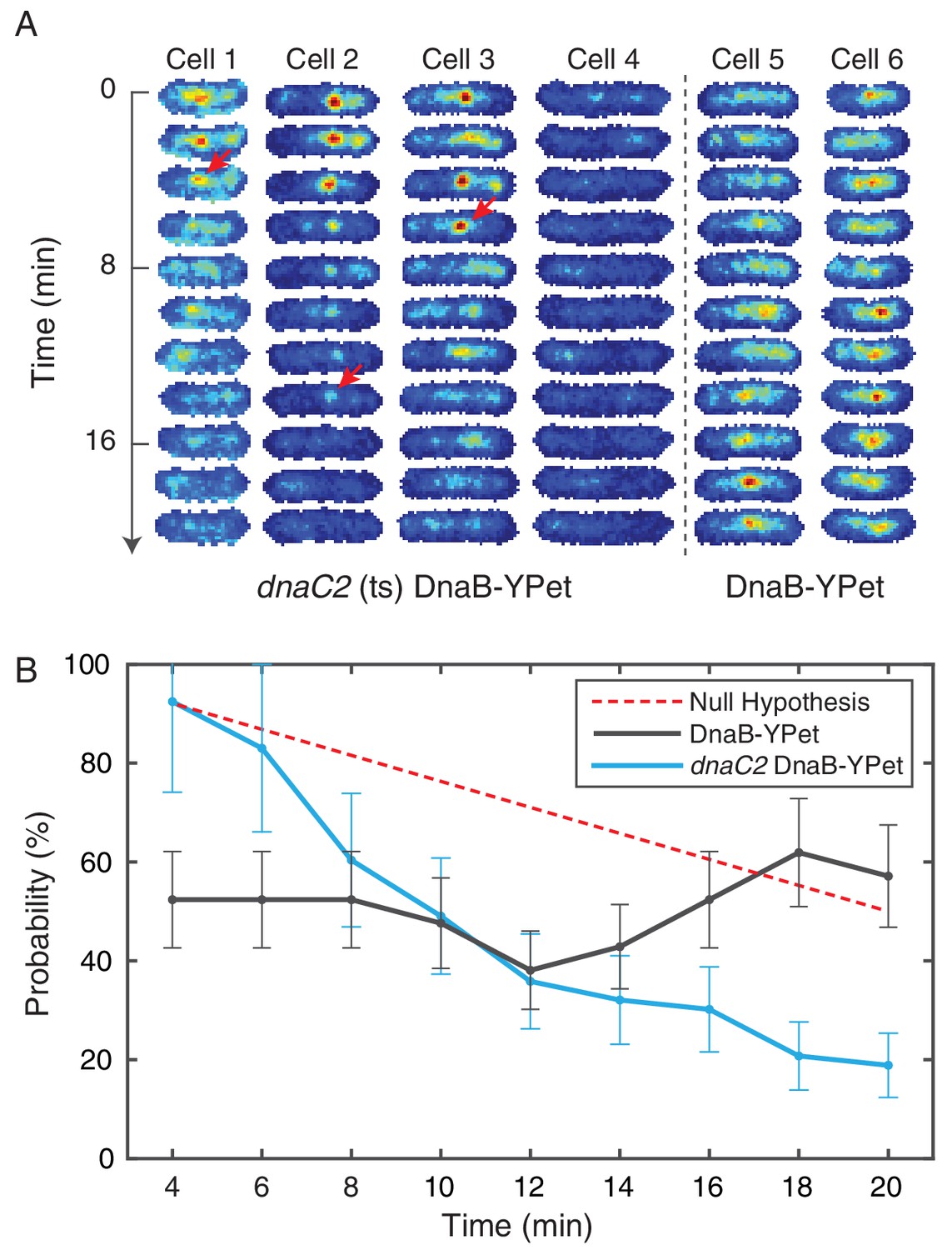
Disruption of restart using temperature sensitive DnaC.
(A) DnaB-YPet imaged at 2 min intervals in strains with and without the dnaC2 allele at 37°C (non-permissive for the temperature sensitive strain). In the temperature sensitive strain, either a complex is observed in the first frame (e. g. cells 1–3) or the cell generally does not develop complexes during the time course (e. g. cell 4). When a complex is observed, it most commonly disappears before the end of the time course. Once disappearance has occurred (red arrows), no new stable complexes are observed in the majority of cells (85%). In contrast, the wild type strain (e. g. cells 5–6) shows intermittent foci (as observed in the dynamics experiments at 30°C), and complexes may be assembled later in the time series. (B) Probability of observing a focus as a function of time in cells where at least one trajectory is observed. DnaC is involved both in initiation of replication at the origin and the rescue of stalled forks. The theoretical ‘Null hypothesis’ curve (red) assumes a continuous 40 min replication cycle imaged for a random 20 min window. However, the probability of observing a focus in the dnaC2 allele (blue, N = 72) decreases more quickly suggesting that the helicase is disassembled prior to completion of replication. Additionally, in the wild type strain, the probability of observing a focus is roughly independent of time, indicating that both disassembly and re-assembly events are present.
Figure 6
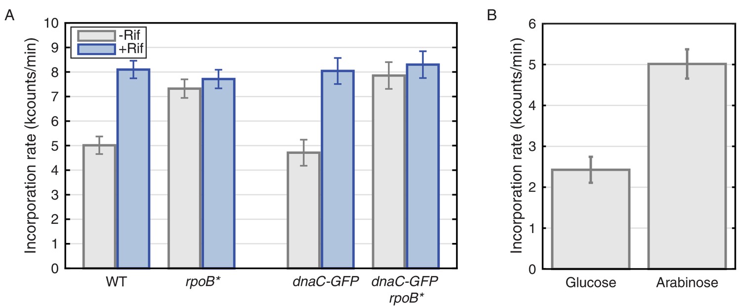
Thymidine incorporation assays determine the effect of transcription on replication rate.
(A) DNA replication rates increase upon transcription-inhibition and in rpoB* strains. Thymidine incorporation assays were used to measure the relative rates of DNA replication in WT and DnaC-GFP strains, with (blue bars) and without (gray bars) perturbations to transcription by rifampicin treatment (Rif) or rpoB* cells. Note that rpoB* strains are resistant to rifampicin and therefore show no additional increase in replication rate after rifampicin treatment. (B) DNA replication rates increase in cells grown in minimal arabinose medium, relative to glucose, where transcription of rRNA and other ribosomal protein genes is higher.
Figure 7 with 5 supplements
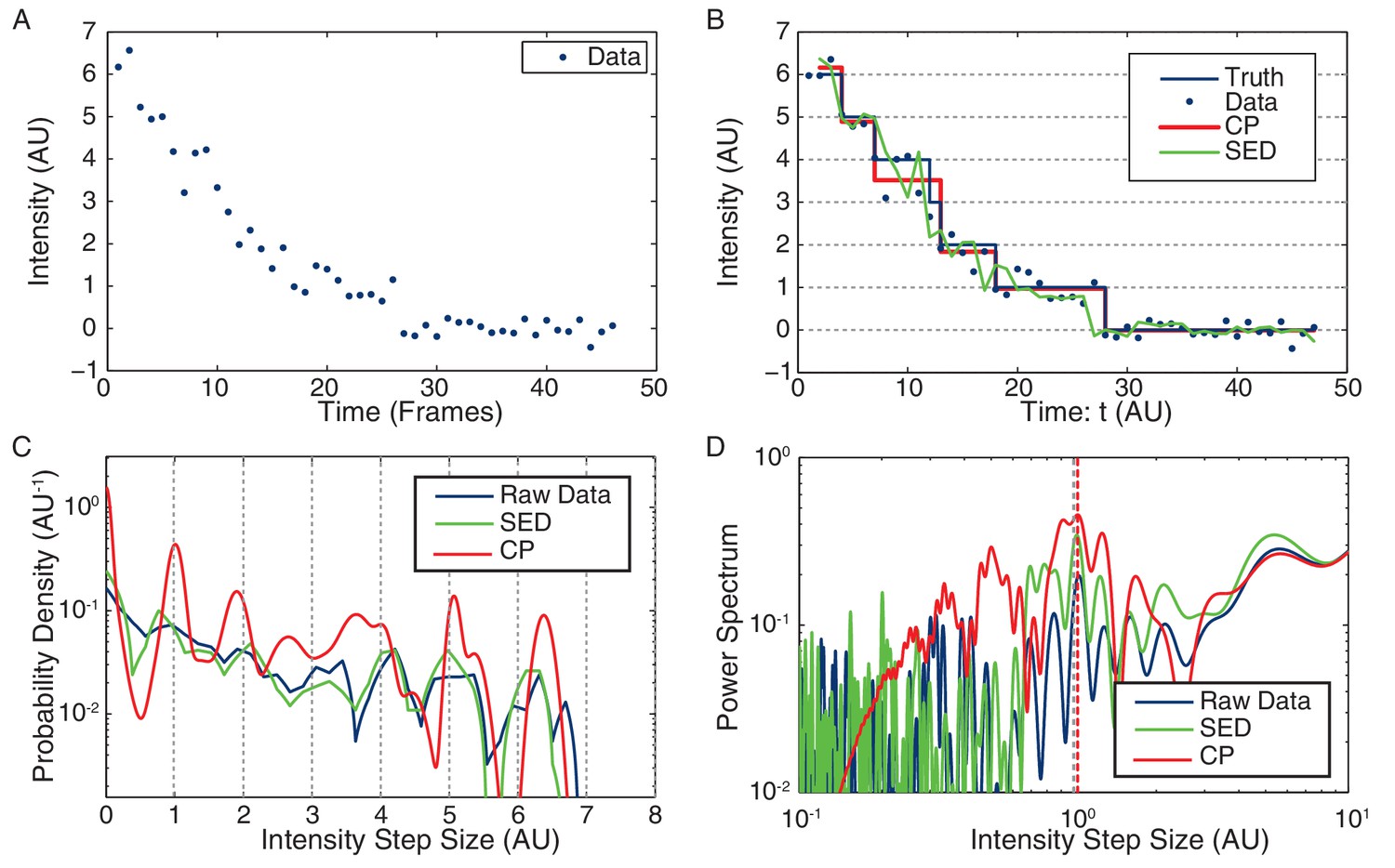
Stoichiometry calculation applied to simulated data.
(A) Simulated intensity data. A bleaching experiment was simulated to demonstrate the performance of the CP Algorithm against the SED filter. The noise and trace length were chosen to closely approximate the observed data. (B) Idealized intensity traces. The data (blue dots) is identical to Panel a. True simulated mean (Truth) is shown in blue. There is excellent agreement between the truth (blue) and the CP idealization (red). The SED filtered trace is shown in green. (C) Pairwise intensity difference probability distribution (PDPD). The black dotted lines represent multiples of the true step-size 1 AU. (D) Power spectrum of the PDPD. The largest peak in the power spectrum is selected as the unitary step (red dotted). The true step-size is also shown (black dotted).
Figure 7—figure supplement 1
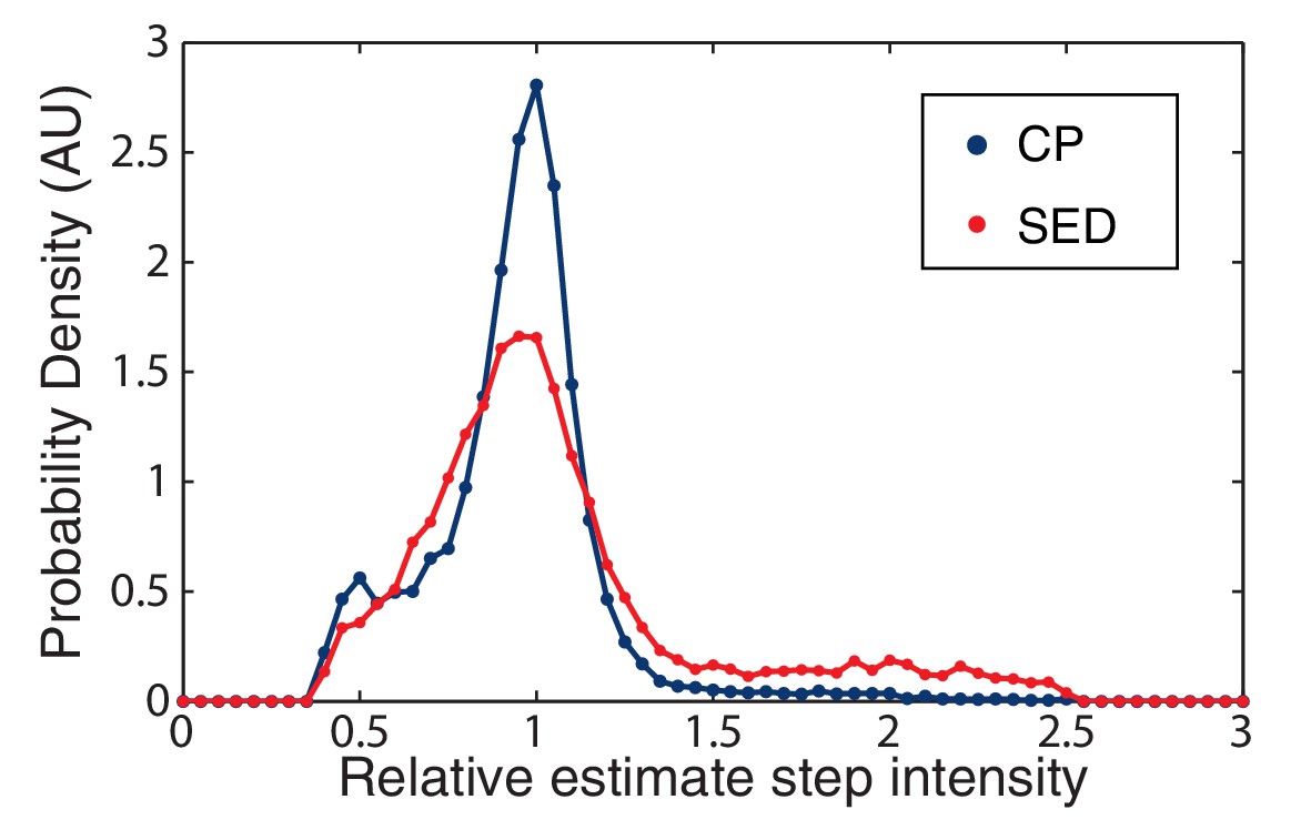
CP versus SED filters in unity step determination.
The performance of the CP versus the SED filter is measured by a histogram of the relative size of the unitary step in simulated data. The CP idealization clearly results in a sharper distribution about the true value (unity).
Figure 7—figure supplement 2
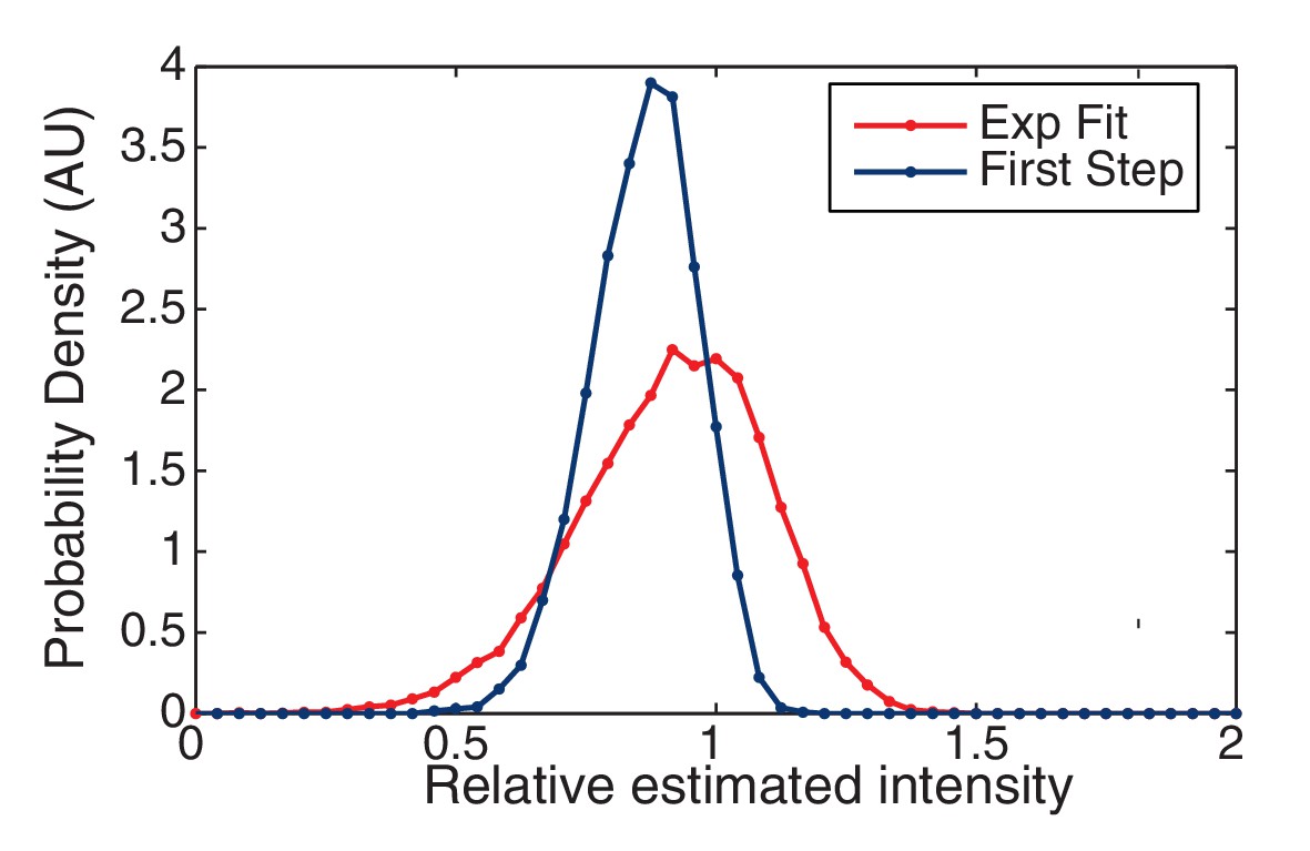
Finding the initial intensity.
We simulated two approaches for determining the initial intensity of the trace: Exponential Fit and Highest-Level. The probability of the estimated intensity is shown relative to the true initial intensity. The Highest Level method is clearly biased from below relative to the Exponential Fit method which is centered around the true value (unity).
Figure 7—figure supplement 3
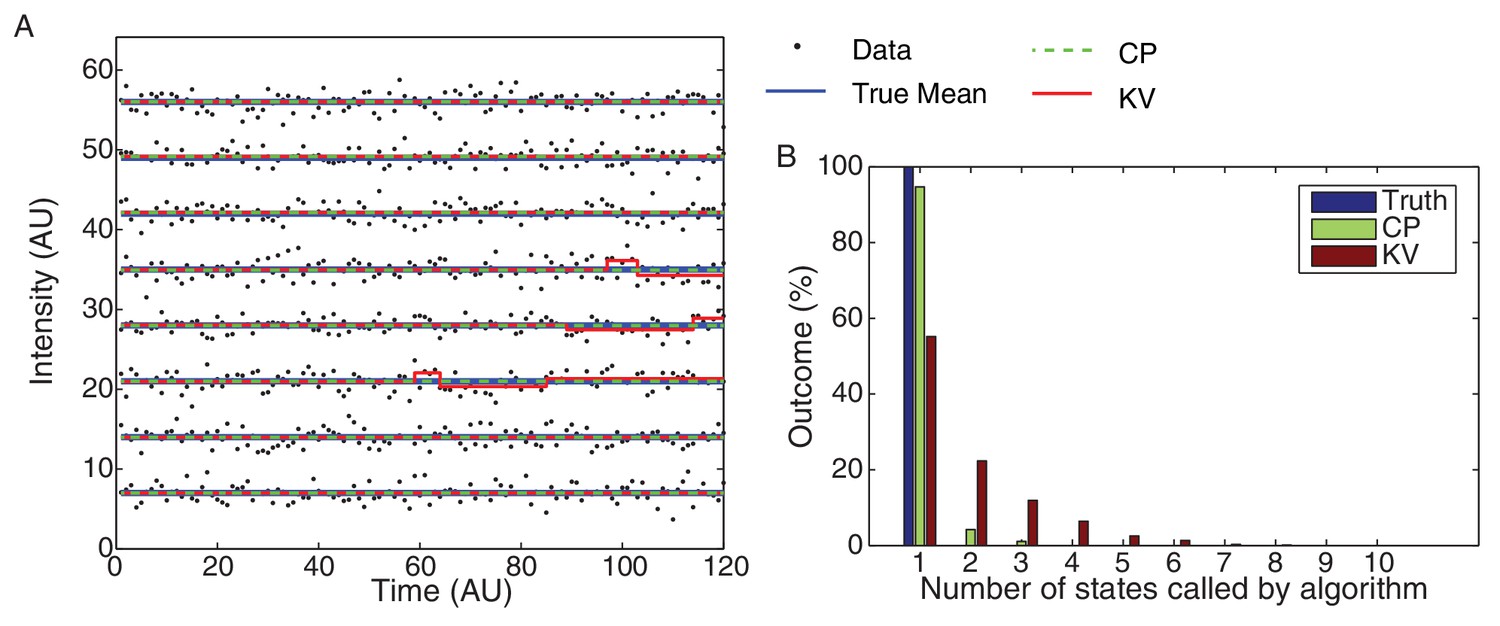
CP vs KV filtering algorithm.
(A) Eight typical datasets (black dots) are plotted with the true mean (blue) and idealizations using both the KV (red) and CP (green) algorithms. The simulated data consisted of 10,000 Gaussian processes with unit variance simulated for 120 frames each. The over segmentation generated by the KV algorithm is clearly visible in the (false) transitions shown in the third, fourth, and fifth traces. No false steps were observed in these eight traces using the CP algorithm. (B) The total number of states for the 10,000 simulated datasets is shown for the true mean and the CP and KV idealization. All datasets consisted of a single true level. The true number of states (one) was found 95% of the time using the CP algorithm and only 55% of the time using the KV algorithm.
Figure 7—figure supplement 4
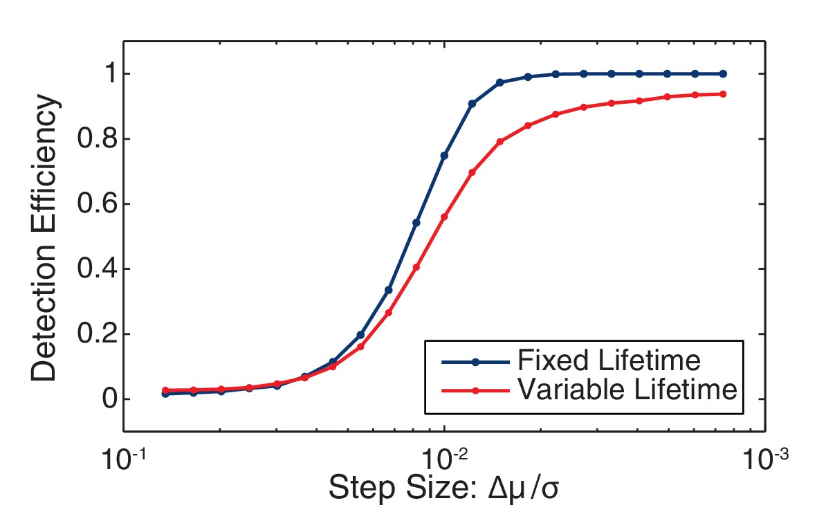
Change point detection efficiency.
The efficiency of change-point detection was measured for fixed-lifetime and variable-lifetime (constant decay rate) steps. In both cases the mean lifetime was equal to the inverse observed decay rate (41 frames). For fixed-lifetime steps (blue), the detection efficiency is essentially unity for relative step-size greater than two. (We define the relative step size as the mean intensity difference divided by the standard deviation: Δµ/σ.) For variable-lifetime steps (red), the detection efficiency is reduced by the existence of a small fraction of short-lived steps.
Figure 7—figure supplement 5
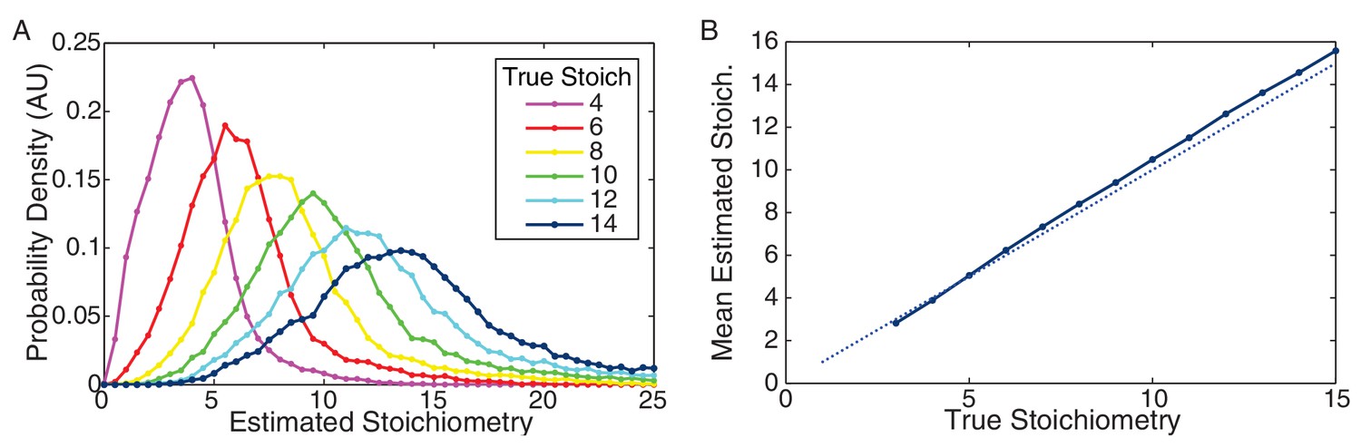
Performance of CP algorithm on simulated data.
(A) Distribution of estimated stoichiometry for simulated data with true stoichiometries from 4–14 proteins. (Integer stoichiometries between 3 and 15 were simulated. For clarity only the distributions for even stoichiometries are plotted.) (B) Mean estimated stoichiometry as a function of true stoichiometry. The estimated stoichiometry slightly overestimates the true stoichiometry (by a fraction of a protein).
Tables
Table 1
Parameters used in B. subtilis complex lifetime calculation. The parameters summarized above are defined as follows: T is the duration of the experiment, is the number of complexes interpreted to disassemble before the end of the experiment, is the number of complexes surviving the length of the experiment, is the minimum observable complex lifetime, is the empirical mean of the observable lifetimes, is the calculated disassembly rate, is the calculated mean lifetime (i.e. ), and is the calculated number of conflicts per 40 min of replication.
T (min) | (min) | (min) | (min-1) | (min) | ||||
|---|---|---|---|---|---|---|---|---|
Wild-Type | 22 | 296 | 31 | 4 | 10.4 | 0.12 | 8.3 | 4.8 |
Rif-Treated | 22 | 86 | 97 | 4 | 12.9 | 0.03 | 29.2 | 1.4 |
rpoB* | 22 | 93 | 72 | 4 | 12.5 | 0.04 | 22.4 | 1.8 |
Table 2
Maximum likelihood fit parameters for B. subtilis count distributions.
N | (copies) | FL (error) | |
|---|---|---|---|
DnaC-GFP | 213 | 6.2,11.2 | 41 (9.1)% |
DnaC-GFP + Rif | 69 | N/A, 12.1 | 0 (14)% |
DnaC-GFP rpoB* | 60 | N/A,11.1 | 0 (10.0)% |
DnaC GFP lacZ off | 108 | 5.6,11.5 | 65 (5.6)% |
DnaC GFP lacZ on | 174 | 6.0, 10.9 | 88 (3.2)% |
DnaC-GFP CD lacZ | 185 | 5.8, 10.2 | 59 (9)% |
DnaC-GFP + IPTG | 261 | 6.3,11.2 | 54 (11)% |
PolC-YPet | 125 | 2.2,4.9 | 47 (13)% |
PolC-YPet +Rif | 117 | N/A, 4.4 | 0 (14)% |
PolC-YPet rpoB* | 81 | N/A, 4.7 | 0 (9%) |
Table 3
Maximum likelihood fit parameters for E. coli count distributions.
N | (copies) | FL (error) | |
|---|---|---|---|
DnaB-YPet | 146 | 6.6, 11.6 | 59 (15)% |
DnaB-YPet + Rif | 53 | N/A, 12.1 | 0 (13)% |
DnaX-YPet | 125 | 2.8, 5.8 | 53 (13)% |
DnaX-YPet + Rif | 154 | 2.8, 5.7 | 10.6 (17)% |
DnaE-YPet | 178 | 2.8, 5.8 | 46 (15)% |
DnaE-YPet + Rif | 144 | 2.8, 5.6 | 9.8 (9.3)% |
Table 4
Parameters used in E. coli complex lifetime calculation. The parameters summarized above are defined as follows: T is the duration of the experiment, is the number of complexes interpreted to disassemble before the end of the experiment, is the number of complexes surviving the length of the experiment, is the minimum observable complex lifetime, is the empirical mean of the observable lifetimes, is the calculated disassembly rate, is the calculated mean lifetime (i.e. ), and is the calculated number of conflicts per 40 min of replication.
T (min) | (min) | (min) | (min-1) | (min) | ||||
|---|---|---|---|---|---|---|---|---|
Wild-Type | 20 | 171 | 46 | 4 | 9.1 | 0.12 | 9.4 | 4.2 |
Rif-Treated | 20 | 42 | 35 | 4 | 12.3 | 0.05 | 21.6 | 1.8 |
Table 5
Strains used in this study.
Strain # | Genotype | Species | Reference |
|---|---|---|---|
HM1 | trpC2 pheA1; wild-type | B. subtilis | Smith et al. |
HM262 | dnaC-gfp-spec | B. subtilis | Lemon et al. |
HM1312 | dnaC-gfp rpoB (H482Y) | B. subtilis | This study |
HM1316 | dnaC-gfp-spec thrC::Pspank(hy)-lacZ::erm | B. subtilis | This study |
HM604 | polC-ypet-mls | B. subtilis | This study |
HM1275 | polC-ypet rpoB (H482Y) | B. subtilis | This study |
HM1500 | lacA::Pxl-dcas9-mls | B. subtilis | Peters et al. |
HM2387 | HM1 lacA::Pxl-dcas9-mls | B. subtilis | This study |
HM2475 | dnaC-gfp-spec amyE::Pveg-sgRNA-priA-cat | B. subtilis | This study |
HM2486 | dnaC-gfp-spec amyE::Pveg-sgRNA-priA-cat lacA::Pxl-dcas9-mls | B. subtilis | This study |
HM1318 | wild-type (AB1157) | E. coli | Dewitt et al. |
HM1319 | dnaB-ypet-kan | E. coli | Reyes-Lamothe et al. |
PAW912 | dnaX-ypet-kan | E. coli | Reyes-Lamothe et al. |
PAW909 | dnaE-ypet-kan | E. coli | Reyes-Lamothe et al. |
PAW542 | dnaC2 thrA::tn10-tet | E. coli | Reyes-Lamothe et al. |
PAW1182 | dnaB-ypet-km dnaC2 thrA::tn10-tet | E. coli | This study |
Table 6
Microscopy parameters.
Laser power at objective (mW) | Exposure time (ms) | Med. background 1st frame (electrons/pixel) | |
|---|---|---|---|
Bleaching (GFP) | 1.3 | 300 | 87 |
Bleaching (YPet) | 0.4 | 300 | 24.1 |
Lifetime (GFP) | 1.1 | 600 | 76 |
Lifetime (YPet) | 0.1 | 600 | 4.5 |
Additional files
-
Supplementary file 1
Independent fork model.
- https://doi.org/10.7554/eLife.19848.038
Download links
A two-part list of links to download the article, or parts of the article, in various formats.
Downloads (link to download the article as PDF)
Open citations (links to open the citations from this article in various online reference manager services)
Cite this article (links to download the citations from this article in formats compatible with various reference manager tools)
Transcription leads to pervasive replisome instability in bacteria
eLife 6:e19848.
https://doi.org/10.7554/eLife.19848


