Protein sorting by lipid phase-like domains supports emergent signaling function in B lymphocyte plasma membranes
- University of Michigan, United States
Figures
Figure 1 with 7 supplements
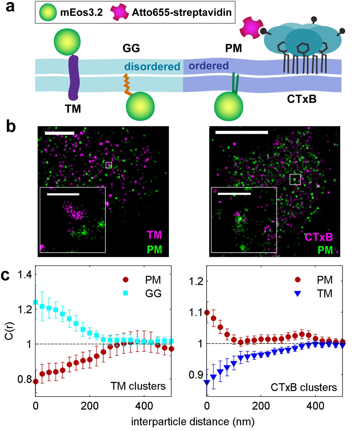
Clusters of ordered or disordered phase markers create distinct membrane domains.
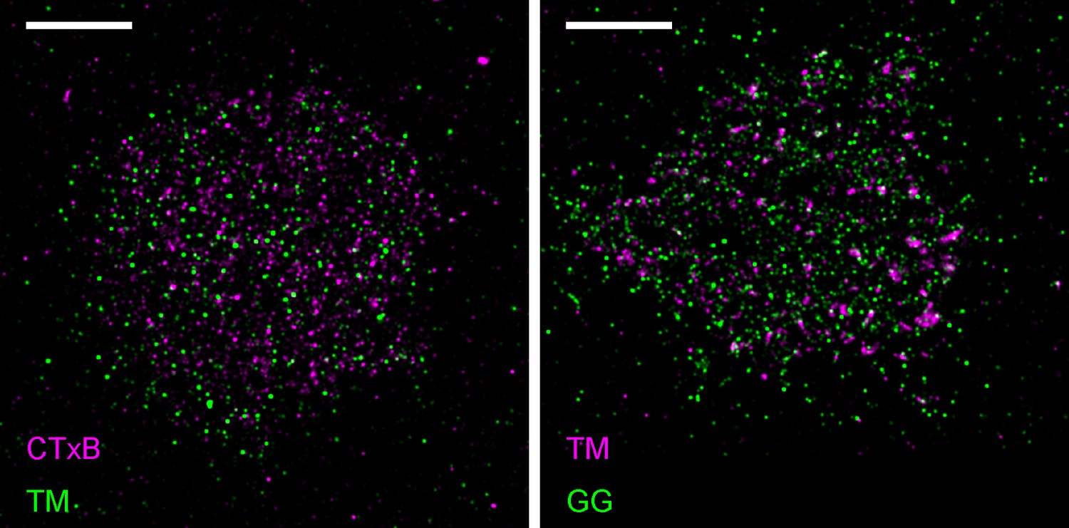
(a) Schematic representation of minimal anchor peptides and their phase preference as determined from model membranes. Amino acid sequences and chemical structures are shown in Figure 1—figure supplement 1. (b) Reconstructed super-resolution images of PM with either clustered TM (left) or clustered CTxB (right). Scale-bars are 5 µm and 500 nm in the inset. (c) Cross-correlation functions, C(r), of PM and GG constructs in cells containing clustered TM (left) or of PM and TM constructs in cells containing clustered CTxB (right). A value of C(r) = 1 indicates a random co-distribution, C(r) > 1 indicates co-clustering, and C(r) < 1 indicates exclusion. These curves represent an average over multiple individual cells from multiple experiments. Curves are averaged over the following number of cells: TM with PM (12) or GG (8), and CTxB with PM (58) or TM (27). Error-bars indicate the SEM between cells. Curves for individual cells are shown in Figure 1—figure supplement 4. Additional representative images for all conditions are shown in Figure 1—figure supplement 7.
Figure 1—figure supplement 1
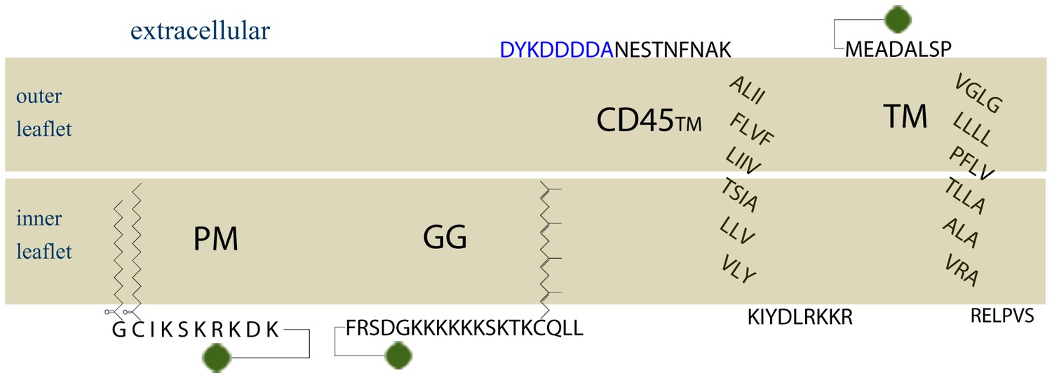
Amino acid sequences of membrane anchors used in this study.
The amino acid sequence and post-translational modification of the four transiently expressed membrane anchors are shown. PM contains the 10 N-terminal amino acids from Lyn, which code for a myristoylation and palmitoylation of the N-terminal glycine and cysteine, respectively. GG contains a polybasic sequence and C-terminal geranylgeranylation, designed from the C-terminal sequence of K-Ras with modification of the CAAX box to code for geranylgeranylation instead of prenylation. CD45TM is the transmembrane domain of CD45 with a FLAG tag, shown in blue, fused to the short extracellular region. Export of CD45TM to the plasma membrane is improved by addition of the signal sequence from HA on the N-terminus. The signal sequence is cleaved in the ER and is not shown here. The full CD45TM sequence is described in the Materials and Methods. TM is the transmembrane domain of Linker for Activation of T Cells (LAT) where palmitoylation sites have been mutated. The fluorophore mEos3.2 is depicted as a green circle, and linker amino acids between the membrane anchors and mEos3.2 are depicted as straight lines.
Figure 1—figure supplement 2
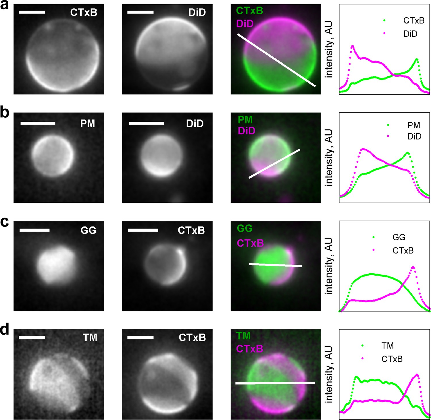
Membrane anchors partition into different phases in GPMVs.
(a) Alexa-555 CTxB and DiD-C16 partition into different phases in GPMVs. CTxB is a well-established marker of the liquid-ordered phase, indicating that DiD-C16 partitions into the liquid-disordered phase. (b) PM-eGFP and DiD C16 partition into alternate phases, indicating that PM-eGFP partitions with the liquid-ordered phase. These GPMVs were prepared with glutathione instead of DTT to preserve the palmitoylation state of this peptide. (c) eGFP-GG and Alexa647 CTxB partition into alternate phases, indicating that GG partitions into the liquid-disordered phase. (d) YFP-TM and Alexa647 CTxB partition into alternate phases, indicating that TM partitions into the liquid-disordered phase. Grayscale images were acquired sequentially for the labels indicated leading to some movement of the vesicle and domains occur between acquisitions. False-colored images represent a simple superposition of the two color channels. The traces at the right denote the fluorescence intensity along the white line shown in the false colored image. In all instances, the vesicle surface was imaged and not a cross-section, leading to fluorescence intensity present in the vesicle interior. The scale bar in all images is 5 µm.
Figure 1—figure supplement 3
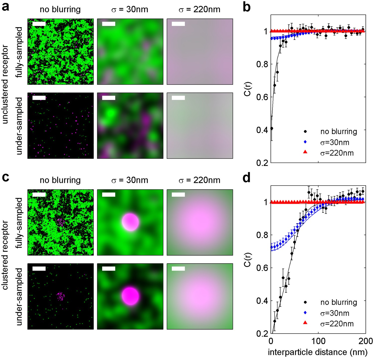
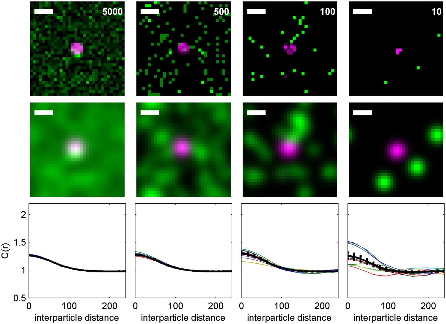
Finite lateral resolution and incomplete spatial sampling impacts measured cross-correlations.
An Ising model simulated at T = 1.05 times the critical temperature is used to demonstrate how finite lateral resolution and incomplete spatial sampling impacts measurements of cross-correlations between proteins and membrane phase-like domains. (a, c) Magenta points represent ordered domain preferring proteins that are either allowed to explore all space (a) or are forced to reside within a circular domain (c). Green pixels in the fully sampled images (top panels of a and c) represent disordered components and black pixels represent ordered components. In the under-sampled images, green points are a subset of the green pixels shown in the fully sampled images, at a density of roughly 400/µm2 (100 points per 512 by 512 nm box). The left-most images in a and c represent simulation snapshots without additional processing. The remaining images are generated from the same information present in the left-most image, but both colors are filtered (blurred) by a 2D Gaussian function with standard deviation (σ) of 30 nm (second column) or 220 nm (third column) to simulate the finite localization precision of super-resolution microscopy or traditional resolution of diffraction-limited microscopy, respectively. Scale-bars are 100 nm. (b, d) Cross-correlations C(r) between magenta proteins and green disordered components were tabulated from 100 images similar to those shown in panels of a and c. Solid lines represent C(r) tabulated from fully sampled images (top panels of a, c) and points with error bounds represent C(r) tabulated from under-sampled images (bottom panels of a, c). Without blurring, it is clearly evident that green components are depleted from the local area around proteins (C(r) < 1 for short separation distances (r) in simulations of both clustered and unclustered proteins. Blurring by the super-resolution localization precision (σ = 30 nm) dramatically reduces the magnitude of depletion in the absence of protein clustering (blue points in b), but depletion is still apparent when proteins are clustered (blue points in d). This is because the size of the protein cluster is on the same order as the length scale of the Gaussian blurring. In contrast, no significant depletion is observed when blurring is applied to mimic conventional fluorescence microscopy (σ = 220 nm) because the length scale of blurring is much longer than the size of protein and membrane phase-like structures. These results visually demonstrate that finite resolution limits reduce the magnitude of observed correlations. Also, in all cases, cross-correlation functions tabulated from under-sampled images reproduce those of the fully sampled images within error bounds even though the images are visually very different. We also note that experimental super-resolution images are not able to accurately capture the fraction of the membrane occupied by one type of phase-like domain. For the example of the unclustered receptor with σ = 30 nm, the fully-sampled image gives the false impression that the majority of the frame is occupied by green (disordered) components, even though it is actually only 50% of the total area. In contrast, the under-sampled image gives the visual impression that less than half of the frame is occupied by green disordered components. Both finite lateral resolution and under-sampling in space make it difficult to accurately determine the surface fraction occupied by phase-like domains in experimentally acquired super-resolution images.
Figure 1—figure supplement 4
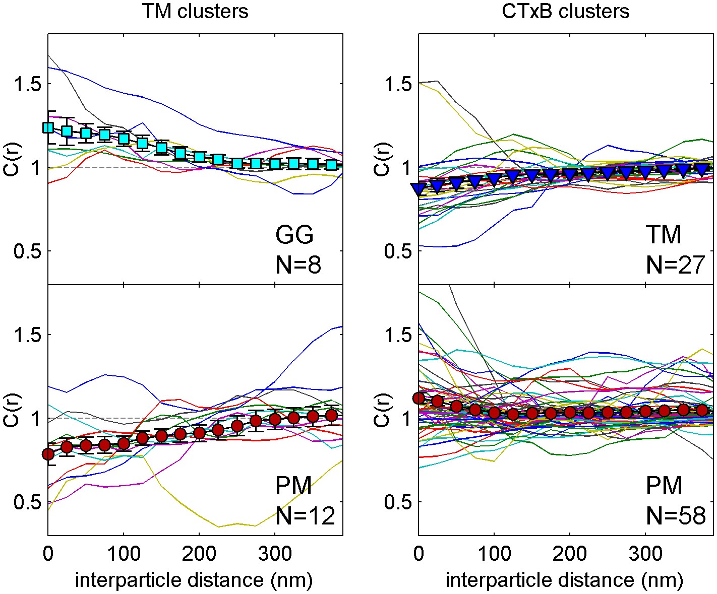
Correlation functions from individual cells and average curves.
Colored lines are cross-correlation curves from individual cells that contribute to the average curves presented in Figure 1c. The large filled symbols represent the average curve and error bars indicate the standard error of the mean between individual curves at each interparticle distance.
Figure 1—figure supplement 5
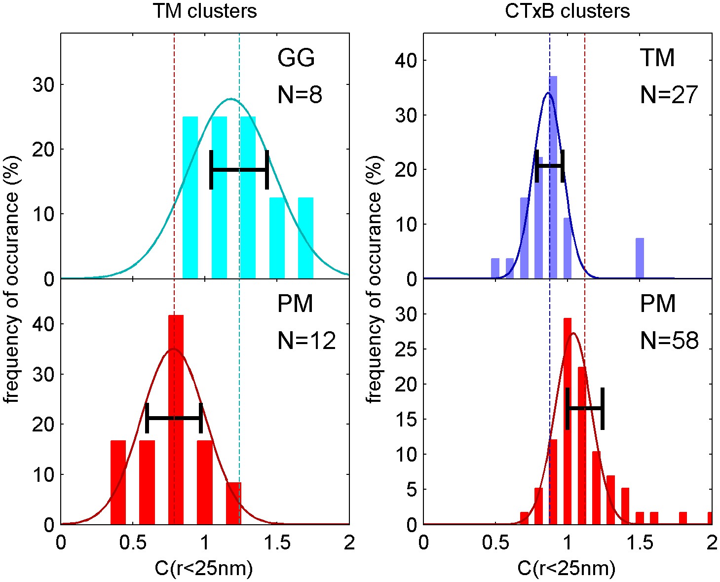
Distribution of correlation function values closely matches the width expected from single measurement errors.
The histograms show the distributions of C(r < 25 nm) values obtained from single cell measurements under each of the conditions indicated. The curved lines indicate the best fit Gaussian function to each histogram, demonstrating that values are normally distributed. The horizontal errorbar is centered around the average value and indicates the magnitude of the average error (dC2) determined by estimating error on single cell measurements of C(r) as described in the Materials and Methods. Since dC2(r) is not calculated for the first spatial bin (r < 25 nm), we instead use the next bin (25 nm < r < 50 nm) for this comparison which likely underestimates the single cell error. The center of this errorbar is placed at the mean value of C(r < 25 nm) which is not always the center of the Gaussian fit. The observation that the average error bar from a single cell measurement is close to the width of the distribution of single cell measurements indicates that errors are dominated by sampling statistics and not by other types of cell-to-cell variation.
Figure 1—figure supplement 6
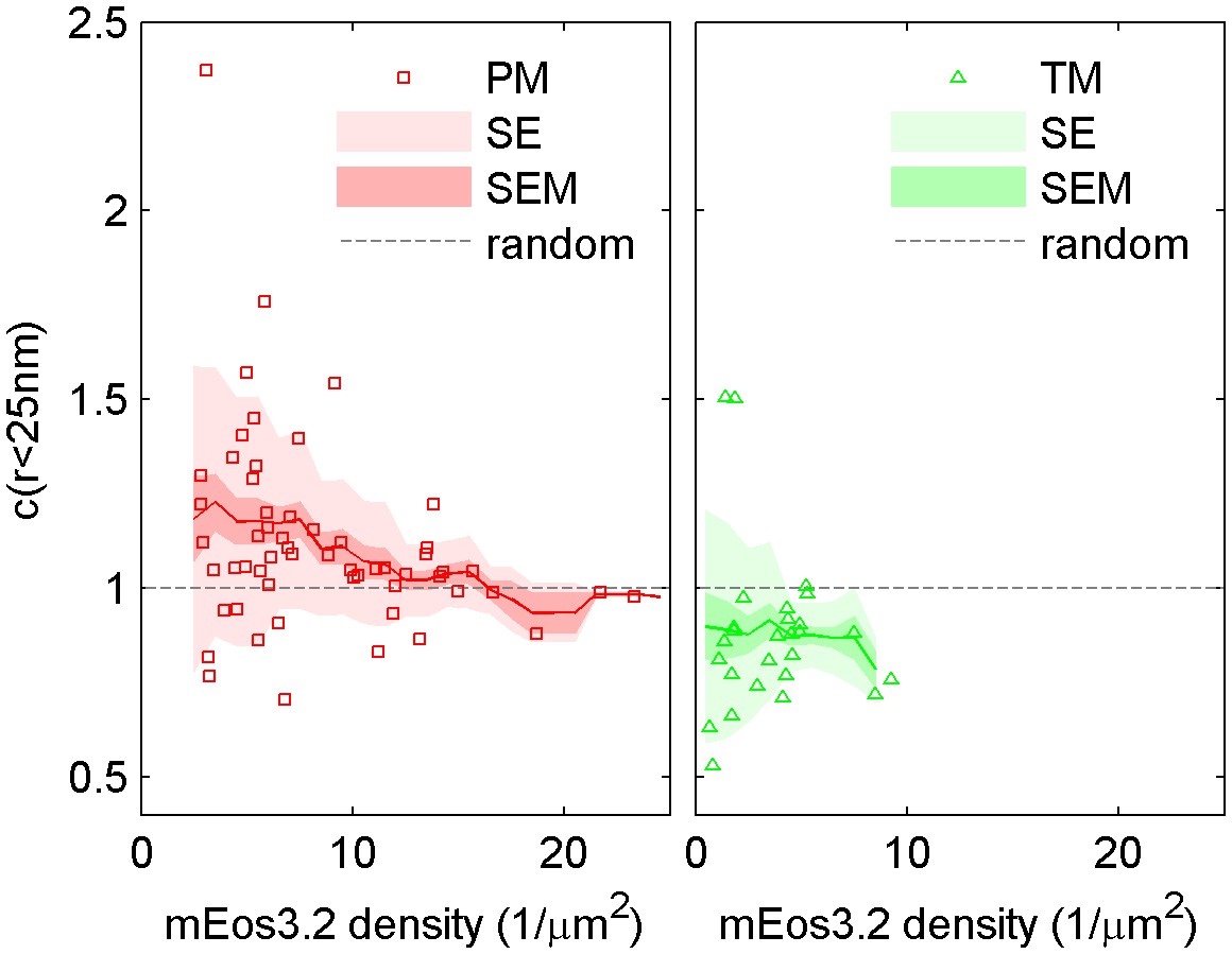
The cross-correlation amplitude is weakly dependent on lipid probe expression level.
The first spatial bin of the cross-correlation C(r < 25 nm) is plotted against the density of the mEos3.2 probe for individual cells. Surface density of mEos3.2 is determined by fitting the autocorrelation as described in Methods. The solid line shows a moving average of the points, the lighter shaded region shows the standard error and the darker shaded region shows the standard error of the mean of C(r < 25 nm). Higher density of lipid probe has negligible effect on TM cross-correlations with clustered CTxB, but has a small effect on PM correlations with clustered CTxB, acting to reduce the cross-correlation at very high densities of mEos3.2 expression.
Figure 1—figure supplement 7
Representative images from Figure 1.
Representative images from conditions included in average curves but not shown in Figure 1. Scale bars are 5 µm. (left) Cells expressing mEos3.2-TM were labeled with CTxB-biotin that was then clustered with streptavidin-Atto655. (right) Cells expressing both mEos3.2-GG and YFP-TM. TM was clustered using a biotinylated anti-GFP antibody followed by streptavidin-Atto655.
Figure 2 with 10 supplements
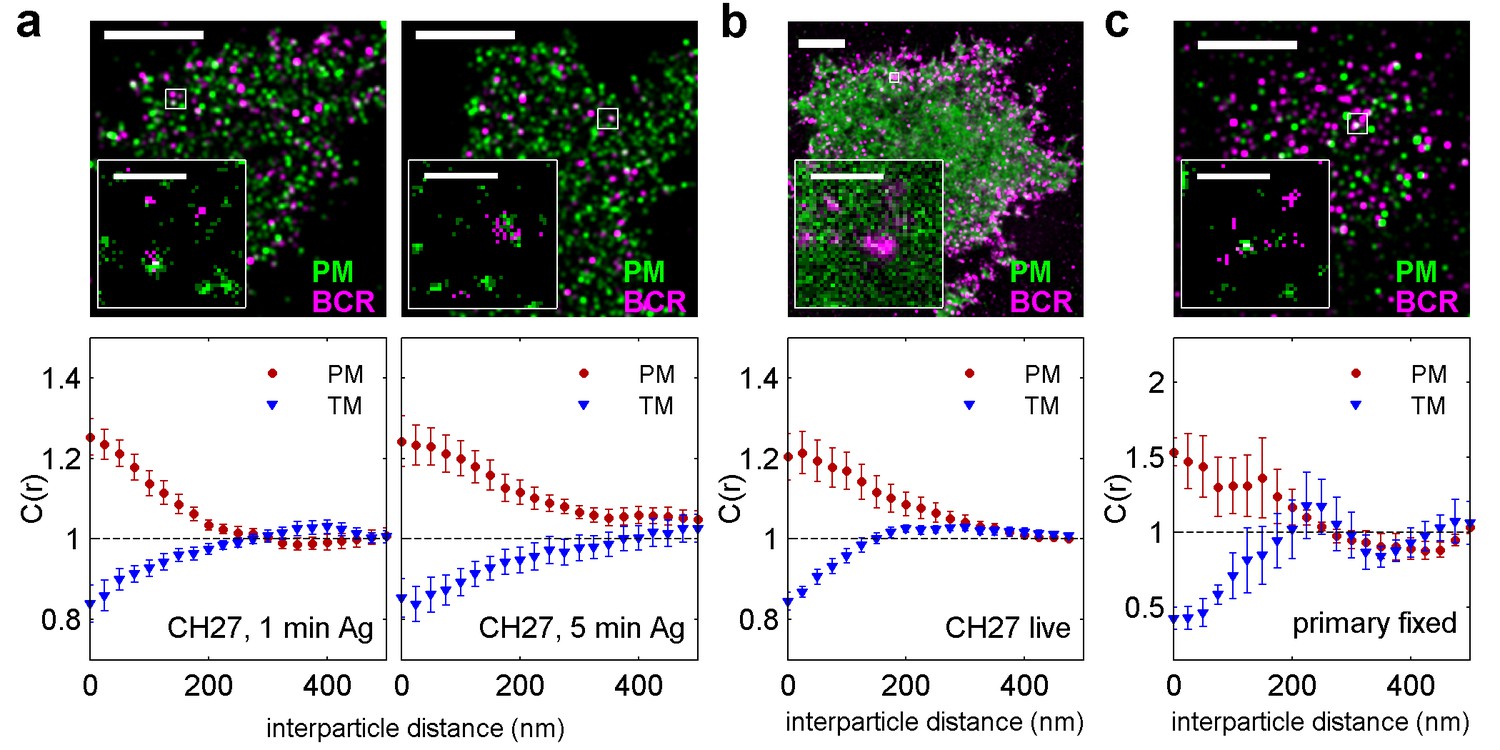
BCR clusters localize within ordered membrane domains.
(Upper panels) Representative reconstructed super-resolution images of the BCR and PM in chemically fixed (a) and live (b) CH27 B cells, and chemically fixed primary B cells (c). Scale-bars are 5 µm and 500 nm in the inset. (Lower panels) Average cross-correlation curves, C(r), between BCR and phase markers. Error-bars indicate the SEM between cells. In (a) cells were chemically fixed either 1 min following BCR clustering (1 min Ag, left) or 5 min after BCR clustering (5 min Ag, right). In (b), data was acquired from live cells between 0 and 6 min following BCR clustering. In (c), BCR was clustered for 5 min prior to chemical fixation. In all cases, the order-favoring peptide (PM) was enriched and the disorder-favoring peptide (TM) was depleted from BCR clusters. Curves from individual cells are shown in Figure 2—figure supplement 1. Curves are averaged over the following number of cells: (a) 1 min BCR and PM (18) or TM (11); 5 min BCR and PM (21) or TM (10). (b) BCR and PM (4) or TM (4). (c) BCR and PM (4) or TM (5). Correlation curves from right column in (a) were used to make a schematic figure showing enrichment and depletion of probes around BCR clusters in Figure 2—figure supplement 4. Representative images for conditions not shown here can be found in Figure 2—figure supplement 10.
Figure 2—figure supplement 1
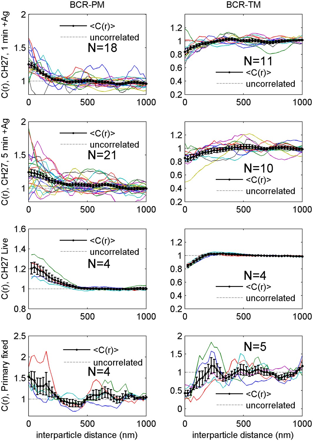
Correlation functions from individual cells and average curves.
Cross-correlation curves from individual cells (colored lines) are averaged to obtain the curves shown in Figure 2 (black lines with errorbars). Error bounds indicate the standard error of the mean between curves at each interparticle distance. Average cross-correlations are computed from the number of cells (N) indicated on each plot.
Figure 2—figure supplement 2
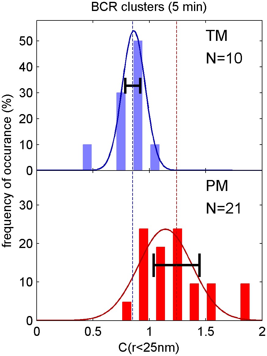
Distribution of correlation function values closely matches the width expected from single measurement errors.
The histograms show the distributions of C(r < 25 nm) values obtained from single cell measurements in fixed cells where clustered BCR was imaged with the anchor probes indicated. The curved lines indicate a Gaussian fit to each histogram, demonstrating that values are normally distributed. The horizontal errorbar is centered around the average value and indicates the magnitude of the average error (dC2) determined by estimating error on single cell measurements of C(r) as described in Methods. Since dC2(r) is not calculated for the first spatial bin (r < 25 nm), we instead use the next bin (25 nm < r < 50 nm) for this comparison which likely underestimates the single cell error. The center of this errorbar is placed at the mean value of C(r < 25 nm) which is not always the center of the Gaussian fit. The observation that the average error bar from a single cell measurement is close to the width of the distribution of single cell measurements indicates that errors are dominated by sampling statistics and not by other types of cell-to-cell variation.
Figure 2—figure supplement 3
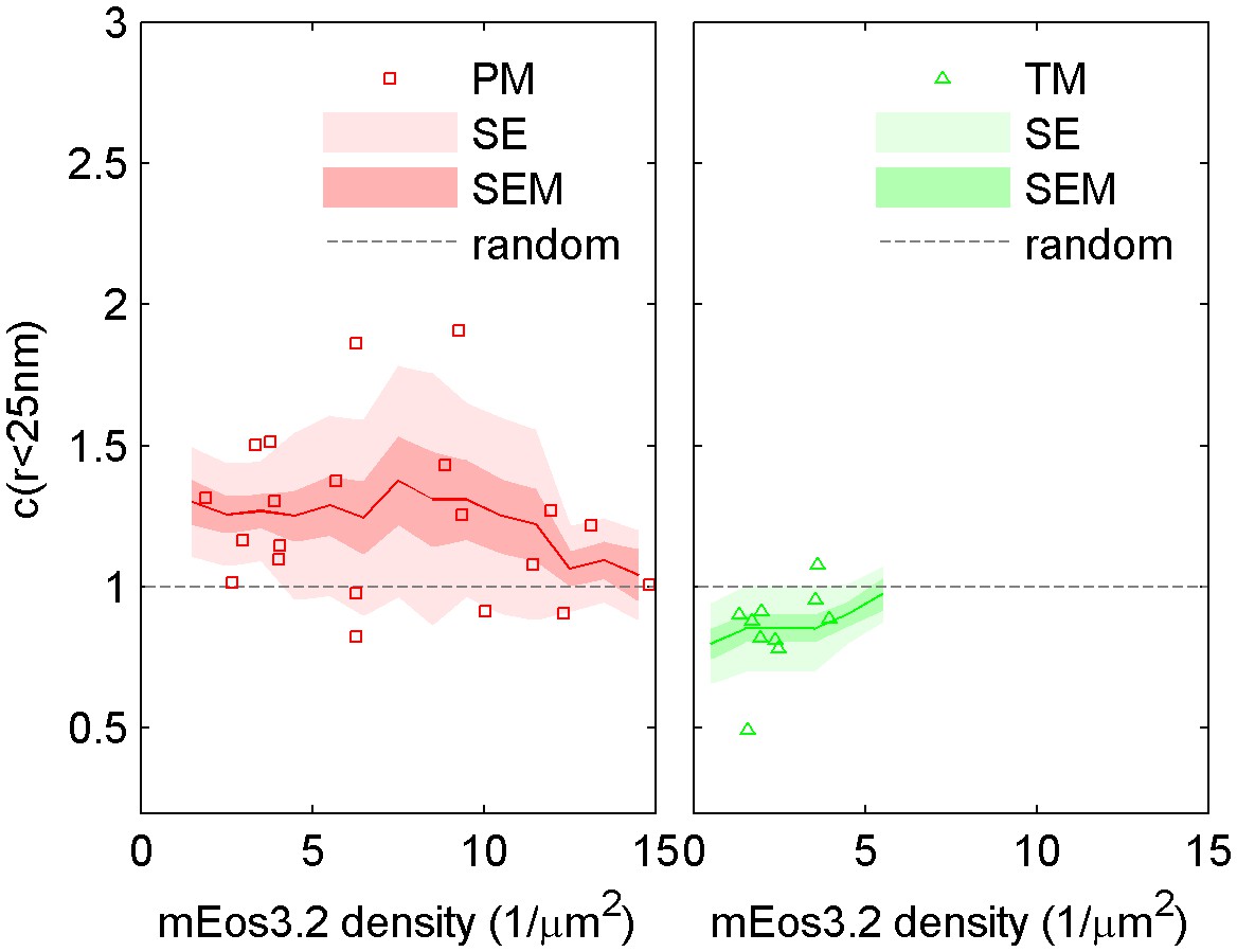
Dependence of cross-correlation amplitudes on lipid probe expression levels.
The first spatial bin of the cross-correlation C(r < 25 nm) is plotted against the density of the mEos3.2 probe for individual cells. Surface density of mEos3.2 is determined by fitting the autocorrelation as described in Methods. The solid line shows a moving average of the points, the lighter shaded region shows the standard error and the darker shaded region shows the standard error of the mean of C(r < 25 nm).
Figure 2—figure supplement 4
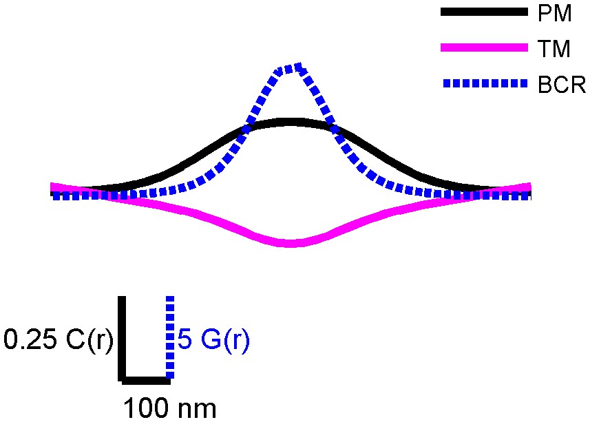
PM and TM cross-correlation functions have a larger correlation length than BCR autocorrelation functions.
Conceptual diagram showing correlation functions from CH27 cells fixed 5 min following BCR clustering that were smoothed and made symmetric about the y axis. This figure highlights the length scale differences between the BCR autocorrelation (blue) and cross-correlations between BCR and PM (black) and TM (magenta). The range of the BCR autocorrelation is a measure of the size of BCR clusters, and BCR correlations with PM and TM extend to larger distances. The magnitude of the BCR autocorrelation is much greater than that of the cross-correlations shown. To facilitate visual comparisons, the vertical scale for the BCR autocorrelation, G(r), is different than the one used for the cross-correlations, C(r), as indicated.
Figure 2—figure supplement 5

Cross-correlations between clustered BCR and PM are reduced in the presence of a signaling inhibitor.
C(r) between PM and BCR in untreated cells and cells treated with 40 µM of the Src kinase inhibitor PP2 and chemically fixed either one minute (a) or five minutes (b) following antigen addition. The number of cells imaged is included in the legend. PM enrichment in BCR clusters is reduced in PP2 treated cells, suggesting that downstream signaling acts to amplify formation of an ordered domain around BCR clusters.
Figure 2—figure supplement 6
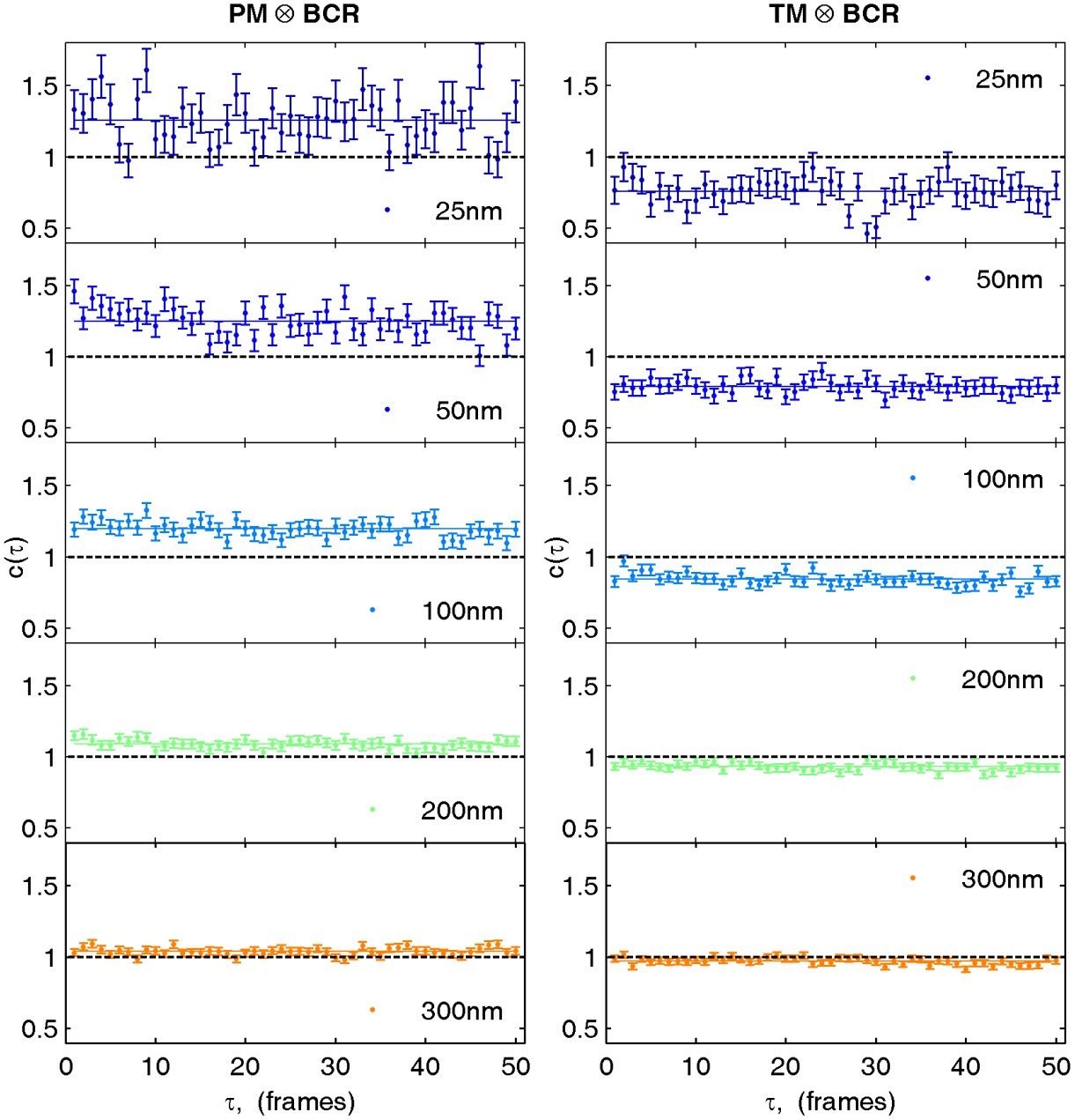
Cross-correlations in live cells are calculated by averaging correlations between non-simultaneous frames.
Cross-correlations between probes in live cells suffer from poor statistics when only simultaneous frames are used to determine the cross-correlation. However cross-correlations between non-simultaneous frames can also be averaged when the time evolution of the cross-correlation is sufficiently slow or predictable. Here, we average correlations for probes observed in the same frame (τ = 0) with correlations from frames shifted in time up to 50 frames (τ = 50) or approximately 1 s. Shown are selected spatial bins from the steady state cross-correlation for clustered BCR with PM (left) and TM (right) from data acquired on a single cell. Since the cross-correlation does not evolve dramatically between τ = 0 and τ = 50, cross-correlation curves are averaged together over this time window.
Figure 2—figure supplement 7
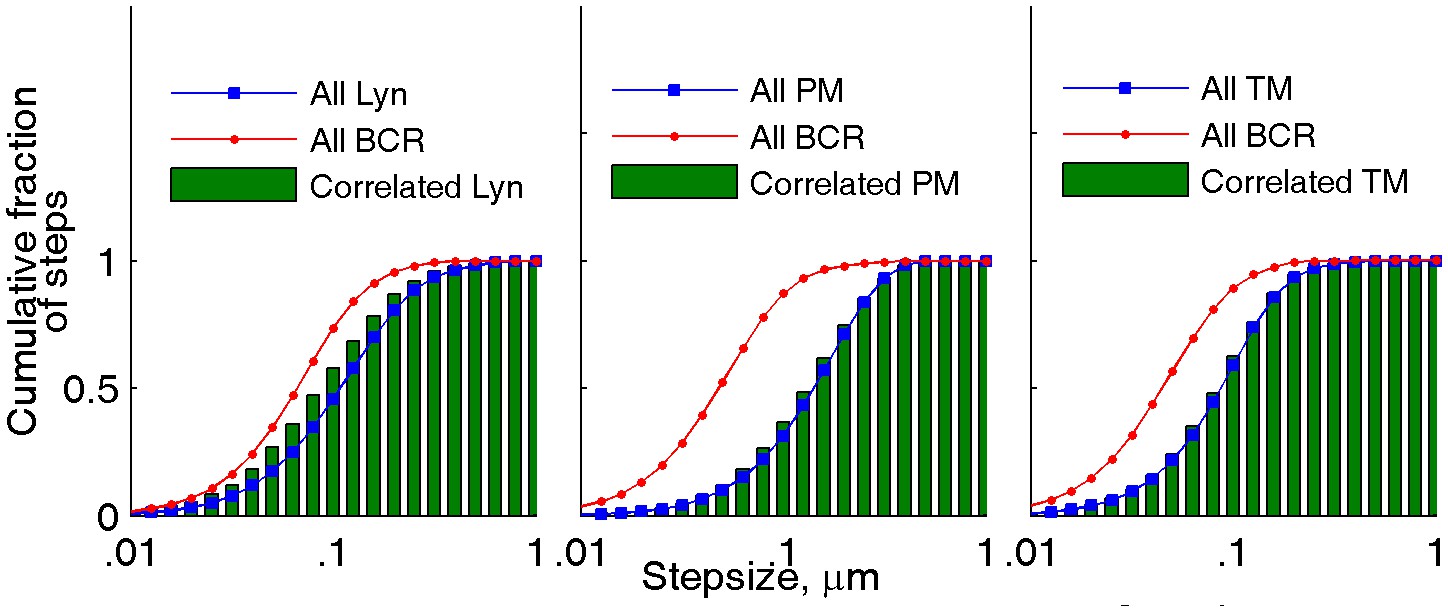
The mobility of lipid probes is not altered when in close proximity to BCR clusters.
The mobility of anchors in close proximity to BCR clusters was probed in the same two-color live cell super-resolution experiments presented in Figure 2. The cumulative step-size distributions shown were either assembled from all steps in probe trajectories (red and blue curves for BCR and anchor probes, respectively) or from the subset of steps in probe trajectories detected within 100 nm of a BCR localization in the same image frame (green bars). Step-sizes for correlated probes were determined from the probe positions in the immediately preceding and following frames. Correlated Lyn diffuses somewhat more slowly than the total population of Lyn, most likely due to binding to BCR. When close to BCR, the lipid probes PM and TM exhibit the same mobility as their respective total populations, indicating that membrane domains do not alter protein mobility at the temporal and spatial scales probed. NLyn = 8, NPM = 14, NTM = 8.
Figure 2—figure supplement 8
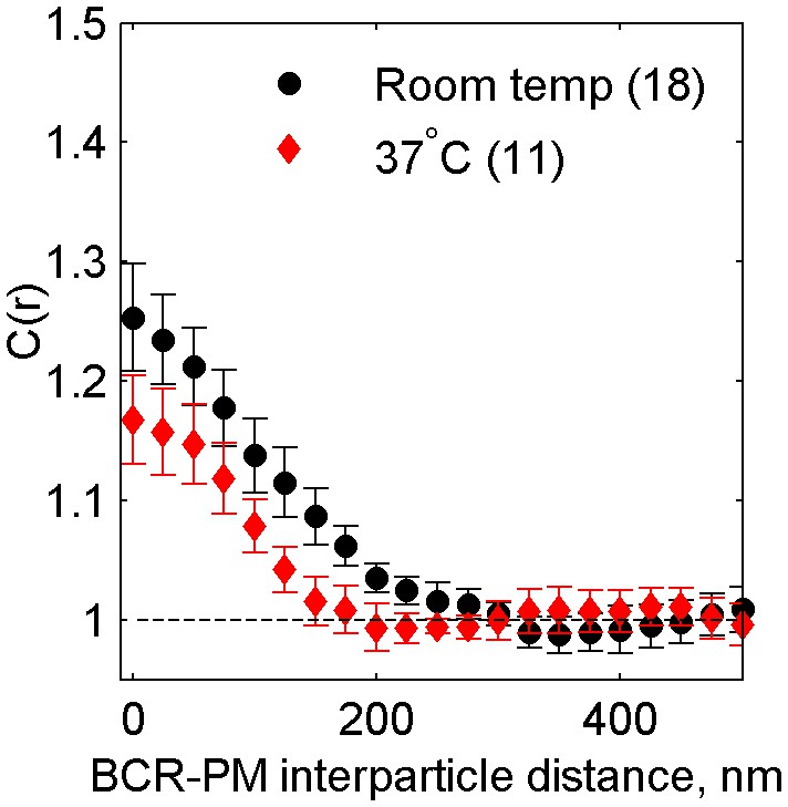
Cross-correlations between clustered BCR and PM are reduced but still observable at physiological temperatures.
Average cross-correlation (C(r)) between PM and BCR at room temperature or at growth temperature (37°C) one minute following antigen addition (NRT = 18, N37 = 11). PM enrichment in BCR clusters is reduced but still present at 37°C, indicating that domains around BCR persist at physiological temperatures.
Figure 2—figure supplement 9

Cross-correlations between PM and unclustered BCR or CTxB are near detection limits.
Representative images (top) showing cells expressing PM-mEos3.2 and labeled with Atto655 anti-IgM f(Ab)1 (left) or Atto655-CTxB (right), where BCR or CTxB labels are not clustered with streptavidin. Scale bars are 5 µm. Average cross-correlations, C(r) (bottom), between unclustered BCR and lipid probes (left) and unclustered CTxB and lipid probes (right). Curves indicate an average over multiple cells (N): BCR and PM (14), CTxB and PM (18). Subtle enrichment of PM is evident in both cases.
Figure 2—figure supplement 10
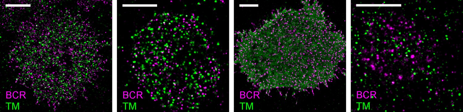
Representative images from Figure 2.
Representative images from conditions included in average curves but for which images are not shown in Figure 2. Scale bars are 5 µm. In all images, IgM BCR is labeled with f(Ab)1 conjugated to Atto655 and clustered with streptavidin. TM is expressed as a mEos3.2 fusion protein. From left to right: CH27 cell fixed 1 min following antigen addition; CH27 cell fixed 5 min following antigen addition; live CH27 cell reconstructed from frames following antigen addition; murine primary B cell fixed 5 min following antigen addition.
Figure 3 with 4 supplements
Ordered domains promote tyrosine phosphorylation.
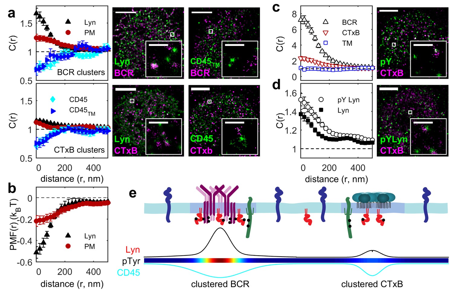
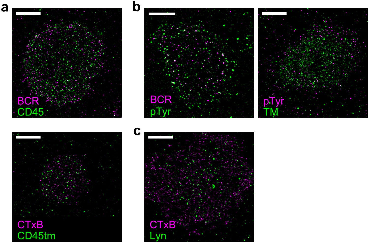
(a) Average cross-correlation functions (C(r), left) and representative super-resolution images (right) demonstrating that full-length proteins and their minimal membrane anchors sort with respect to clusters of both BCR (top) and CTxB (bottom). The correlations presented represent an average over multiple (N) individual cells: Between BCR and Lyn (4), PM (21), CD45 (10), CD45TM (10); between CTxB and Lyn (19), PM (58), CD45 (11), and CD45TM (5). (b) Lyn and PM distributions with respect to B cell receptor clusters expressed as the potential of mean force (PMF). (c) Both BCR and CTxB domains are sites of tyrosine phosphorylation (pY) as detected through a generic anti-pY antibody (4G10), while disordered TM domains were not enriched in pY proteins. Curves are averaged over the following number of cells: BCR and pY (14), CTxB and pY (13), and TM and pY (7). (d) Activated Lyn (pY-397) was more enriched in CTxB clusters than Lyn as a whole, indicating that ordered domains favor activation of this protein. Curves are averaged over the following number of cells: CTxB and pY Lyn (40), CTxB and Lyn (49). (e) Schematic of membrane domains stabilized by BCR and CTxB clusters. Curves and color-scale at bottom are quantitative representations of the relative enrichment or depletion of the components indicated as represented in parts a and c. Scale-bars are 5 µm and 500 nm in the inset. Additional representative images are shown in Figure 3—figure supplement 4.
Figure 3—figure supplement 1
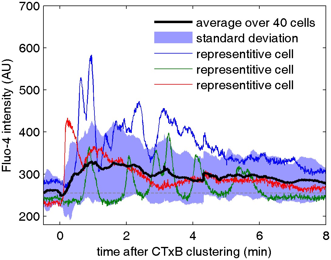
Cell surface clustering of cholera toxin subunit B elicits calcium mobilization in B cells.
Cytosolic calcium levels were monitored in CH27 B cells both before and after biotinylated CTxB was clustered with streptavidin using the calcium indicator Fluo-4 as described in Methods. Colored curves represent raw fluorescence intensity traces for single cells and the average response of 40 cells is shown in black. The blue shaded region denotes +/- one standard deviation between the averaged cells. One reason for the broad width of this distribution is that individual cells oscillate between high and low fluorescent states, as apparent in the single cell traces.
Figure 3—figure supplement 2

CTxB clusters are not highly correlated with BCR.
Average cross-correlation between clustered CTxB and BCR indicates that these two proteins are not colocalized. Biotinylated CTxB was clustered by streptavidin conjugated to Atto 655 and cells were fixed prior to labeling BCR with a f(Ab)1 fragment conjugated to Alexa 532. The lack of pronounced cross-correlation between BCR and clustered CTxB indicates that CTxB is not forcing BCR to be clustered nor was it strongly recruiting BCR. Interestingly, the weak enrichment of BCR within CTxB clusters is similar to the enrichment of membrane anchored probes around clustered CTxB and BCR, suggesting that the enrichment stems from domain partitioning. The curve is an average of 6 cells with errorbars showing the standard error of the mean.
Figure 3—figure supplement 3
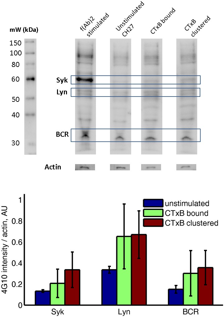
Subtle increases in protein phosphotyrosine levels in response to CTxB clustering are suggested by western blots of whole cell lysates.
CH27 cells were treated as indicated above lanes, and anti-phosphotyrosine western blots were performed using cell lysates. The top shows a representative western blot, where identity of Syk, Lyn, and BCR bands are estimated from the molecular weight marker shown at right. The actin band was determined by stripping and reblotting for actin. The bottom shows the quantification of four western blots from two biological replicates, where band intensity was background subtracted and normalized by the actin intensity for that lane. Results are suggestive of increased phosphorylation of BCR, Lyn, and Syk following CTxB binding and clustering although none of the conditions reach p=0.05 significance levels when probed using a two sample t-test. Errorbars show standard error of the mean between the four blots.
Figure 3—figure supplement 4
Representative images from Figure 3.
Representative images from conditions included in average curves in Figure 3 are shown here. Scale bars are 5 µm. (a) Cells stained for CD45 (top) or expressing CD45tm (bottom) where either BCR (top) or CTxB (bottom) was clustered. Average curves are shown in Figure 3a. (b) Phosphotyrosine (pTyr) was immunolabeled in cells where either BCR (left) or TM (right) was clustered. Average curves are shown in Figure 3c. (c) Lyn was immunolabeled in CH27 cells where CTxB was clustered. Average curves are shown in Figure 3d.
Figure 4 with 1 supplement
A model linking receptor clustering to receptor phosphorylation.
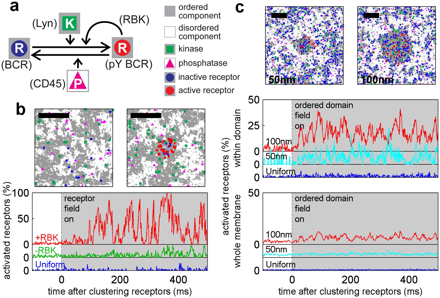
(a) Schematic representation of the model described in the main text. Possible biological analogs of model components are indicated, with “RBK” representing receptor-bound kinases. (b) Simulation snap-shots (top) and sample receptor phosphorylation time-traces (bottom) indicate receptors are robustly phosphorylated (pY) upon clustering when membranes are heterogeneous. Phosphorylation was diminished in simulations without RBKs and absent in simulations with a uniform membrane. All curves have the same vertical scale and time-lapses of the simulations are in Videos 4–6. (c) Simulation snap-shots (top) and sample receptor phosphorylation time-traces (bottom) for simulations where an ordered domain is stabilized without confining receptors to the domain. In this case, more receptors are included to represent the large number of membrane proteins containing tyrosine residues that can be phosphorylated. The efficiency of receptor phosphorylation depends on the size of the stabilized ordered domain for reasons discussed in the main text. All curves have the same vertical scale. Time-lapses of the simulations are shown in Videos 7–9. All scale bars are 100 nm.
Figure 4—figure supplement 1

Simulations naturally reproduce experimental kinase and phosphatase distributions with respect to the BCR.
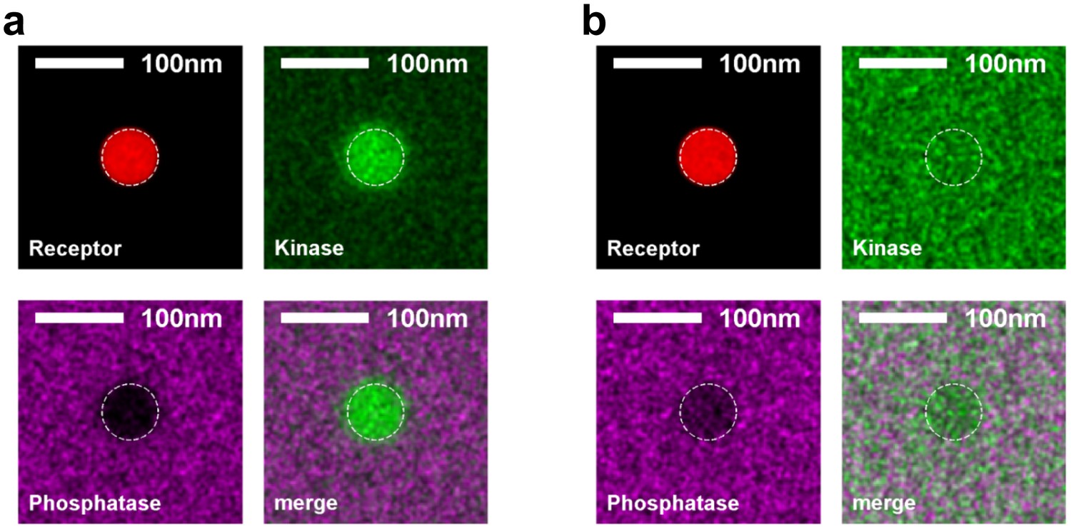
(a) Time-averaged positions of the receptor, kinase, and phosphatase in simulations. Kinases are recruited and phosphatases are excluded from clustered BCR. The location of the receptor cluster is indicated by the dashed white line. (b) Average cross-correlation functions between unclustered receptors (top) or clustered receptors (bottom) and kinases and phosphatases from simulation snap-shots. On the right, simulation images are convolved with a Gaussian function with a 30 nm standard deviation prior to conducting the cross-correlation to better mimic experimental conditions.
Figure 5 with 3 supplements

Phosphorylation model predicts the response to changing the fraction of ordered and disordered components.
(a) Representative snap-shots (top) and histograms showing receptor phosphorylation (bottom) in simulations run with different fractions of ordered and disordered components (grey and white pixels respectively). Receptors (not shown) were confined within the red dashed circle. Snap-shots corresponding to conditions in the plot are indicated as colored symbols. (b) Cross-correlations between receptors and ordered components in simulations run with a variable fraction of ordered and disordered components. Simulations shown are a subset of those displayed in (a) as indicated by symbols. (c) Acute cholesterol modulation with MβCD altered the surface fraction of ordered (dark) and disordered (bright) phases in isolated GPMVs (top) and modulated calcium mobilization in response to antigen, measured using the cytoplasmic Ca2+ indicator Fluo-4 (bottom). Values were normalized to the maximum response of untreated cells. Colored symbols on vesicle micrographs and plot indicate equivalent treatments in both measurements. Calcium measurements are an average of at least two biological replicates. (d) Cross correlations between BCR and PM-mEos3.2 in CH27 cells treated with indicated amounts of MβCD (18), cholesterol-loaded MβCD (18), or left untreated (21) and then fixed 5 min following antigen addition. Scale bars are 100 nm in simulations and 5 µm in micrographs.
Figure 5—figure supplement 1
Kinase and phosphatase partitioning into receptor clusters change dramatically as the surface fraction of ordered components is varied.
Time-averaged positions of the receptor, kinase, and phosphatase in simulations with ordered components making up 20% (a) or 80% (b) of the simulated membrane. The location of the receptor cluster is indicated by the dashed white line.
Figure 5—figure supplement 2
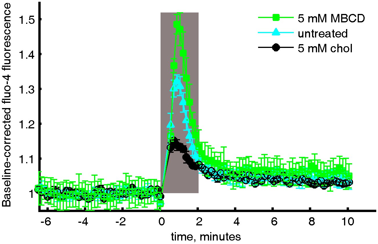
Averaged and baseline-corrected Fluo-4 intensity curves.
Relative Fluo-4 intensity of CH27 cells stimulated with anti-IgM f(Ab)2 with either MβCD treatment, cholesterol treatment, or no treatment. The curves were integrated within the gray box to give the values shown in Figure 5c in the main text.
Figure 5—figure supplement 3
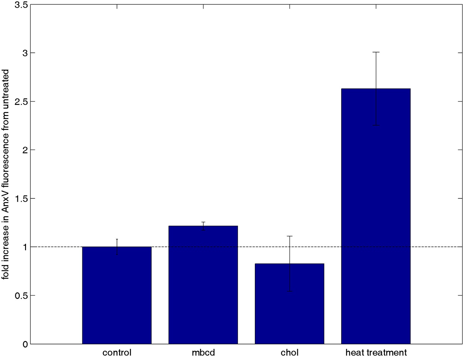
Cholesterol treatments do not alter annexin V staining.
CH27 cells were treated with either 10 mM MβCD, 10 mM MβCD loaded with cholesterol, or control buffer in an identical manner as cells from Figure 3c where calcium release was tested. A positive control was also performed by heat treating cells at 60°C for 15 min. Following treatment, cells were washed and stained with annexin Vconjugated to Alexa 488, which binds to PS on the external leaflet of the plasma membrane when cells are beginning to undergo apoptosis. Cells were washed again after binding to remove unbound annexin Vand total fluorescence was measured using a fluorescence plate reader. The minimal difference in annexin staining between cholesterol treated and untreated cells indicates that the calcium release results shown in Figure 5c are not attributable to changes in cell viability.
Figure 6 with 5 supplements
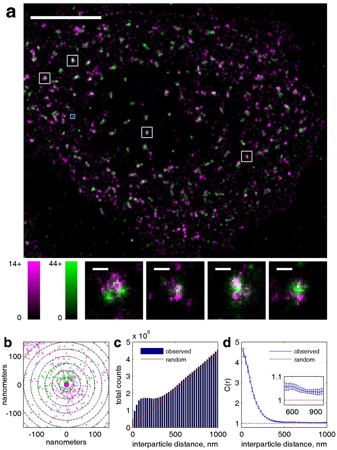
Our cross-correlation methodology applied to doubly labeled clathrin.
(a) Two-color super-resolution image of a HeLa cell expressing two distinct labeled clathrin heavy chain constructs is shown. Clathrin heavy chains associate strongly in clathrin coated pits, and thus serve as an example of highly correlated co-clustered objects. Individual clathrin coated pits are shown below in the smaller images. Scalebar in large image is 5 µm, scale-bars in small images are 200 nm. (b) Zoom in of cyan box shown in large image, where position of points are plotted around an arbitrarily chosen central magenta localization. Dotted lines show the spatial bins used for calculating the cross-correlation function, where the number of green localizations within each bin are counted. In the complete cross-correlation these counts would also be summed over all magenta localizations. (c) Raw histograms of interparticle distances containing all pairs of particles localized within this cell. The red line shows the expected number of pairs in each spatial bin given a random distribution of both magenta and green localizations. The raw histogram is normalized by this curve to yield c(r). (d) Cross-correlation derived from localizations within this cell. Magnitude of the correlation indicates fold increase of pairs detected at the specified inter-particle distance compared to a random distribution. The expected value of the cross-correlation given a random co-distribution is equal to one due to the normalization. Error bounds shown are dC2(r) and are estimated from the statistics and resolution of the image as defined in Equation 3.
Figure 6—figure supplement 1
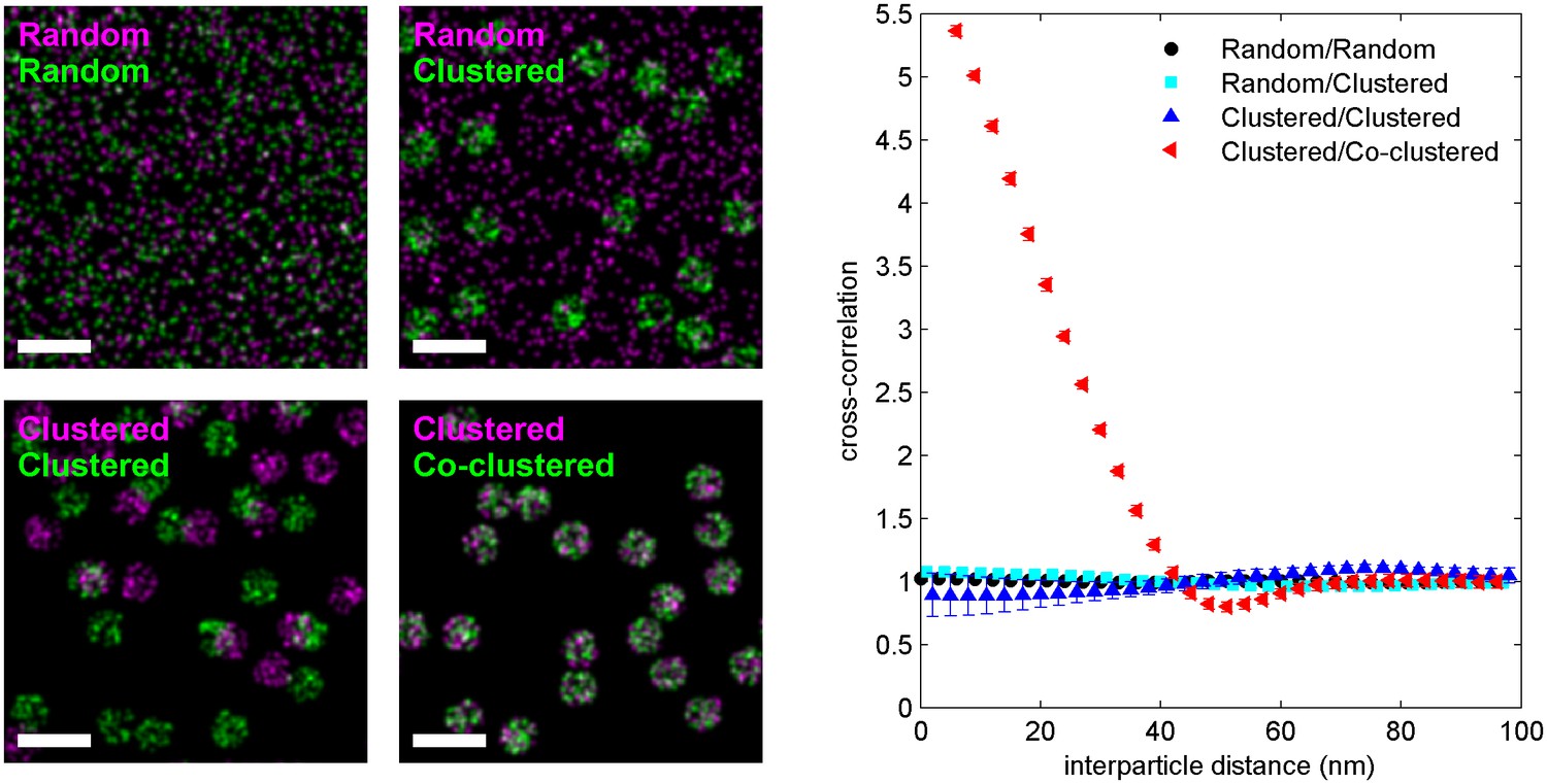
The cross-correlation function detects deviations in the co-distribution of localizations from random.
Four simulations of two-color localization distributions are shown, where the spatial distribution of the localization is given by the labels in the top left of the images. For clustered distributions, particles are randomly placed within non-overlapping circular areas. For co-clustered, both green and magenta localizations are placed within the same circular areas. Cross-correlation functions calculated from simulated distributions are shown at right. Only co-clustered objects yield a cross-correlations that is significantly different from a random distribution. Clustering one object and leaving the other randomly distributed or clustering both objects but maintaining a random co-distribution yields distributions of interparticle distances that are not significantly different than a random co-distribution of both localizations. Scale bars are 100 nm.
Figure 6—figure supplement 2
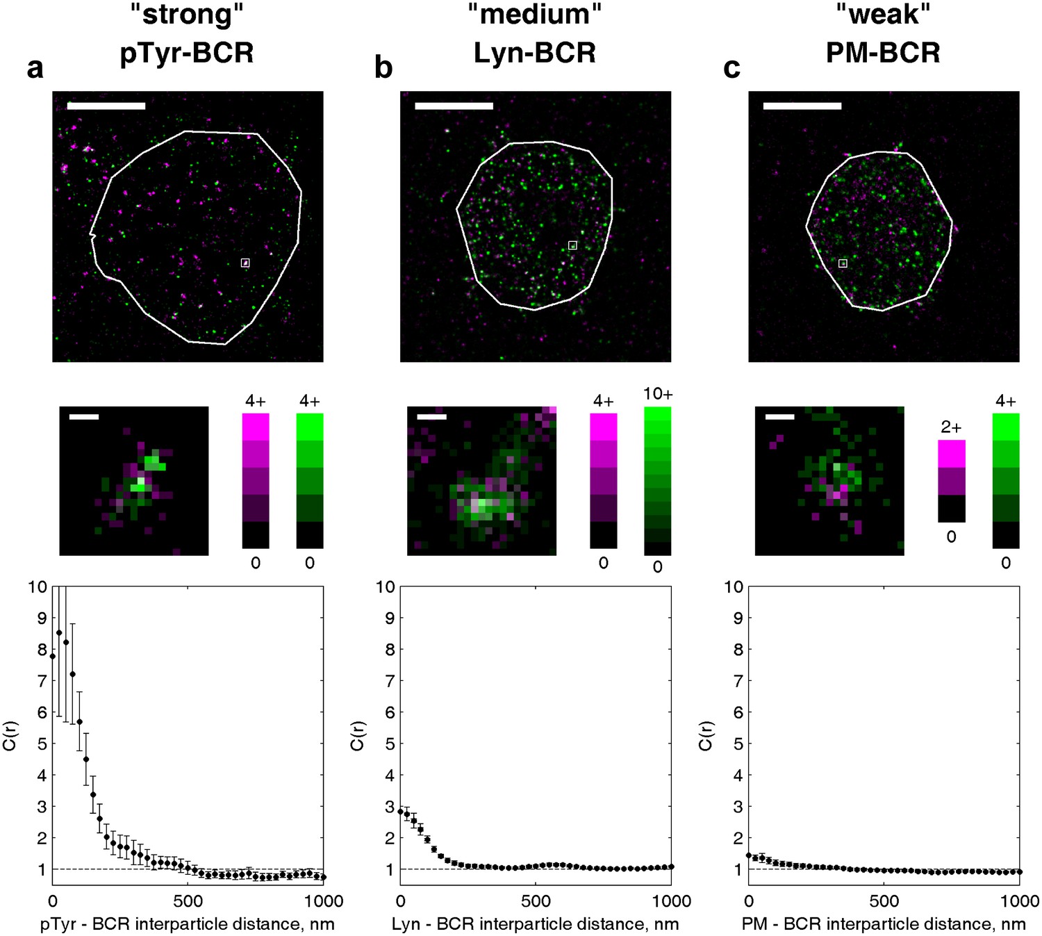
The amplitude of the cross-correlation reflects differences in enrichment magnitude and interaction strength.
Example cells from three different experiments are shown to illustrate the range of values the cross-correlation function can take for various types of interactions. (a) An example of a strong enrichment is shown for phosphotyrosine (pY) and BCR. Nearly every BCR cluster is colocalized with pY localizations, and little pY is observed outside BCR clusters. (b) Lyn transiently binds to phosphorylated ITAMs within BCR clusters but is also present outside of clusters, leading to a reduced magnitude of the correlation function. (c) PM is weakly enriched in BCR clusters and a large fraction of PM is found outside of BCR clusters, however PM is more colocalized than expected from a random distribution when the whole cell is analyzed. In whole-cell images (top), scale bars are 5 µm. Boxed regions shown in whole-cell images are enlarged below (middle) and the number of localizations in each pixel is given by the colorbars. Scale bars in enlarged regions are 100 nm.
Figure 6—figure supplement 3
Cross-correlations detect co-clustering even when there is a low surface density of labeled molecules.
An Ising model containing kinase (green) and clustered receptors (magenta) is used to demonstrate how the surface density of labeled proteins impacts correlation functions. (top) Representative histograms indicating simulated positions of kinase and receptors, with each pixel corresponding to 16 nm × 16 nm area. The average surface density per µm2 is shown. (middle) The same image as above but blurred by a Gaussian function mimicking the localization precision. All scale bars are 100 nm. (bottom) Averaged cross-correlation functions for the conditions represented above. The black curve shows an average over 1000 samplings of the same distribution with the average surface density indicated for both kinase and receptor. The colored lines show averages over 100 samplings. If there are roughly 100 receptor clusters per cell, then these curves represent the expected cell-to-cell variation. Most experiments have mEos3.2 surface expression between 1–20 per µm2 so are expected to most closely mimic the situation on the far right. Note that even when surface densities are low, the average correlation function remains unchanged beyond differences in signal to noise.
Figure 6—figure supplement 4

Membrane topology gives rise to long-range structure in cross-correlations, but can be removed by careful selection of regions of interest (ROI).
(a) Reconstructed super-resolution image of a CH27 B cell in which part of the cell has detached from the coverslip surface leading to a reduction in localizations in the center of the cell, which is imaged in total internal reflection. Two different regions of interests are shown, with the excluded regions lightened for contrast. Scale bars are 5 µm. (b) Cross-correlation functions tabulated using the two ROIs shown in a. The loose ROI produces a C(r) that is correlated and decays slowly with radius. This is largely a reflection of the topology of the ventral membrane, which contains large regions where both probes are excluded due to membrane detachment. This correlation is removed by selecting a ROI which only includes flat regions. (c) ROI generation is performed by users and has the potential to introduce bias into the analysis. 19 cells comprising different labeling and treatment conditions were randomly viewed by users that lacked knowledge of the specific identity of each cell. The three users tended to define masks that yielded correlation functions with similar amplitudes from single cells. (d) Average cross-correlation curves corresponding to the 19 cells shown in d, with errorbars indicating the SEM between cells for each user. These results overlap within error bounds suggesting that arbitrary user decisions regarding ROI placement do not significantly impact this result.
Figure 6—figure supplement 5
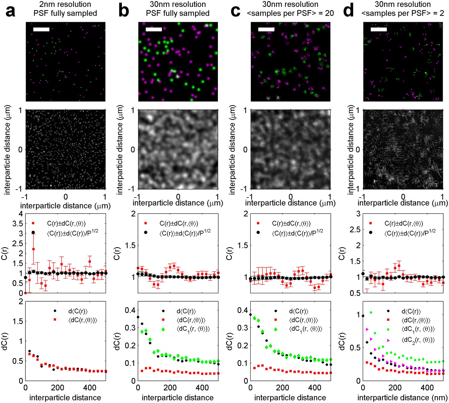
Estimation of the variance associated with a cross-correlation measured on a single super-resolution fluorescence localization image.
Simulations containing randomly distributed green and magenta points are used to identify the sources of error typically found in cross-correlations tabulated from images acquired using super-resolution localization microscopy. Here, labeled molecules are distributed randomly as shown in (a). When the localization precision (30 nm) is on the order of the pixel size (25 nm), then it acts to blur the image of molecular centers (b). The smooth blurred image represents a fully sampled PSF. In real localization microscopy images, single labeled molecules are typically localized multiple times, but not often enough to fully sample the super-resolved PSF. Instead the distribution represented by the blurred image is under-sampled. The smooth shape of the PSF is still evident when each PSF is sampled many times (c), but images appear more pixelated as this sampling is reduced (d). All of these factors impact the statistics of measured correlation functions. For all conditions indicated, the top panel shows a representative simulation snapshot for the condition indicated (scale-bar = 500 nm) and the two dimensional cross-correlation, C(r, θ), tabulated from this representative image. The next lower panel shows C(r, <θ>) obtained by averaging C(r, θ) over angles (red squares), as well as <C(r)>, the correlation function obtained by averaging over 100 simulation replicates (black circles). Error bars on these curves are either determined from the angular average as described in the main text (red squares, dC(r, <θ>)), or by taking the SEM over 100 simulation replicates to obtain d<C(r)> (black circles). The bottom panels show how the square root of the variance (dC(r)) depends on radius for the conditions indicated. Black circular points show (d<C(r)>). Red squares show the dC(r, <θ>) error averaged over the 100 replicates <dC(r, <θ>)>. The dC1(r) and dC2(r) points are corrections to dC(r, <θ>) and are calculated as described in Methods. (a) dC(r, <θ>) is a good estimate of d<C(r)> in simulations where the localization precision is much less than the pixel size and when there is good sampling of the super-resolved PSF. (b) dC(r, <θ>) under-estimates d<C(r)> when labeled objects are detected with 30 nm localization precision but when these super-resolved PSFs are fully sampled. This under-estimate can be corrected using the dC1(r) described in Equation 2 of Methods. (c) dC1(r) is sufficient when labeled objects have 30 nm resolution and their super-resolved PSF is well sampled. (d) An additional correction is needed when the super-resolved PSF is not well sampled, as described by dC2(r) in Equation 3 of Methods.
Videos
Video 1
Reconstructed image time lapse of single molecule localizations from live cell measurements of BCR (magenta) and PM (green).
Individual images are reconstructed using 100 frames (2 s) of single molecule images, receptors are crosslinked at time = 0, and the scale-bar is 5 µm. Single BCR or PM proteins are imaged over multiple frames and each produce clouds of localizations whose extent depend on the protein mobility as well as the typical time that a probe remains activated. This combined with under-sampling of the molecules that are present gives rise to the self-clustered appearance of probes (especially BCR) prior to receptor clustering. Overall, there is not an obvious reorganization of PM after BCR is clustered.
Video 2
Reconstructed image time lapse of single molecule localizations from live cell measurements of BCR (magenta) and TM (green).
Individual images are reconstructed using 100 frames (2 s) of single molecule images, receptors are crosslinked at time = 0, and the scale-bar is 5 µm. Single BCR or TM proteins are imaged over multiple frames and produce clouds of localizations whose extent depend on the protein mobility as well as the typical time that a probe remains activated. This combined with under-sampling of the molecules that are present gives rise to the self-clustered appearance of probes (especially BCR) prior to receptor clustering. Overall, there is not an obvious reorganization of PM after BCR is clustered.
Video 3
Reconstructed image time lapse of single molecule localizations from live cell measurements of BCR (magenta) and Lyn kinase (green).
Individual images are reconstructed using 100 frames (2 s) of single molecule images, receptors are crosslinked at time = 0, and the scale-bar is 5 µm. Single BCR or Lyn proteins are imaged over multiple frames and produce clouds of localizations whose extent depend on the protein mobility as well as the typical time that a probe remains activated. This combined with under-sampling of the molecules that are present gives rise to the self-clustered appearance of probes (especially BCR) prior to receptor clustering. A population of Lyn is immobile or diffuses more slowly. These proteins appear as brighter spots since numerous localizations occur in the same location.
Video 4
Simulated time course of receptor activation upon clustering in a heterogeneous membrane.
Simulations are conducted as described in Methods. The positions of receptors (circles), kinases (green squares), and phosphatases (magenta triangles) are shown at 1 ms intervals (representing 1000 simulation updates). Inactive receptors are shown in blue and activated (phosphorylated) receptors are shown in red. Symbols are drawn larger than the pixels that they represent for clarity. The receptor field is turned on at time = 0 to induce receptor clustering. The time trace shown at the bottom is redrawn from Figure 4b.
Video 5
Simulated time course of receptor activation upon clustering in a heterogeneous membrane without the positive feedback loop accomplished through receptor bound kinases.
Simulations are conducted as described in Methods. The positions of receptors (circles), kinases (green squares), and phosphatases (magenta triangles) are shown at 1 ms intervals (representing 1000 simulation updates). Inactive receptors are shown in blue and activated (phosphorylated) receptors are shown in red. Symbols are drawn larger than the pixels that they represent for clarity. The receptor field is turned on at time = 0 to induce receptor clustering. The time trace shown at the bottom is redrawn from Figure 4b.
Video 6
Simulated time course of receptor activation upon clustering in a uniform membrane.
Simulations are conducted as described in Methods. The positions of receptors (circles), kinases (green squares), and phosphatases (magenta triangles) are shown at 1 ms intervals (representing 1000 simulation updates). Inactive receptors are shown in blue and activated (phosphorylated) receptors are shown in red. Symbols are drawn larger than the pixels that they represent for clarity. The receptor field is turned on at time = 0 to induce receptor clustering. The time trace shown at the bottom is redrawn from Figure 4b.
Video 7
Simulated time course of receptor activation upon stabilization of a large ordered domain.
Simulations are conducted as described in Methods. The positions of receptors (circles), kinases (green squares), and phosphatases (magenta triangles) are shown at 1 ms intervals (representing 1000 simulation updates). Inactive receptors are shown in blue and activated (phosphorylated) receptors are shown in red. Symbols are drawn larger than the pixels that they represent for clarity. The field is turned on at time = 0 to induce a circular ordered domain with a radius of 100 nm. The time trace shown at the bottom is redrawn from Figure 4c.
Video 8
Simulated time course of receptor activation upon stabilization of a small, ordered domain.
Simulations are conducted as described in Methods. The positions of receptors (circles), kinases (green squares), and phosphatases (magenta triangles) are shown at 1 ms intervals (representing 1000 simulation updates). Inactive receptors are shown in blue and activated (phosphorylated) receptors are shown in red. Symbols are drawn larger than the pixels that they represent for clarity. The field is turned on at time = 0 to induce a circular ordered domain with a radius of 50 nm. The time trace shown at the bottom is redrawn from Figure 4c.
Video 9
Simulated time course receptor activation state within a uniform membrane with an applied field.
Simulations are exactly as described for Video 7 but unspecified membrane components are all of the same type (ordered in this case). The positions of receptors (circles), kinases (green squares), and phosphatases (magenta triangles) are shown at 1 ms intervals (representing 1000 simulation updates). Inactive receptors are shown in blue and activated (phosphorylated) receptors are shown in red. Symbols are drawn larger than the pixels that they represent for clarity. The field is turned on at time = 0 but does not impact the organization of components. The time trace shown at the bottom is redrawn from Figure 4c.
Download links
A two-part list of links to download the article, or parts of the article, in various formats.
Downloads (link to download the article as PDF)
Open citations (links to open the citations from this article in various online reference manager services)
Cite this article (links to download the citations from this article in formats compatible with various reference manager tools)
Protein sorting by lipid phase-like domains supports emergent signaling function in B lymphocyte plasma membranes
eLife 6:e19891.
https://doi.org/10.7554/eLife.19891


