Excitation and inhibition in anterior cingulate predict use of past experiences
Figures
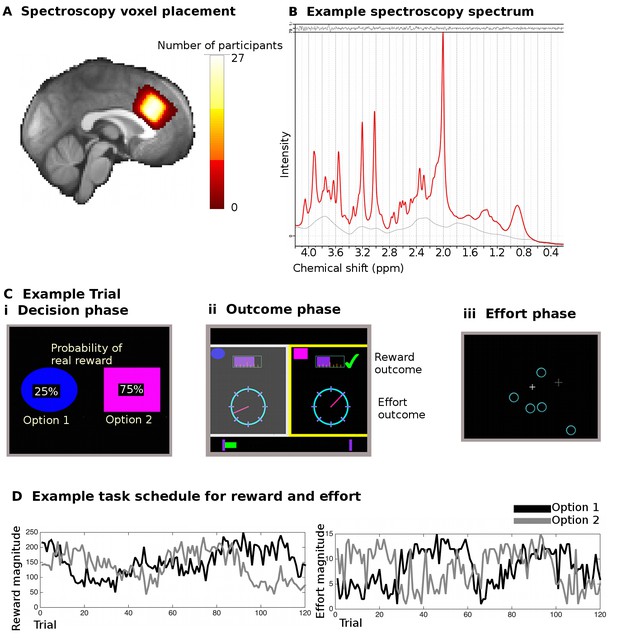
Spectroscopy measurements and task.
(A) Spectroscopy voxels were placed in dACC. Cingulate sulcal morphology was used to guide voxel placement and this resulted in consistent positioning of the voxel in the same location in MNI space (white color indicates overlap in voxel position in all 27 participants). (B) Example spectroscopy spectrum from one participant. The fitted LCModel (red) is plotted overlaid on the actual data (black). The difference between the data and the model (residuals) is shown at the top and the baseline at the bottom. (C) Participants performed 240 trials of a reward- and effort-guided learning task. On each trial, participants were shown two options overlaid with the probability of receiving a reward for each choice (Ci). Participants chose between the options on the basis of the reward probabilities displayed on the screen and on the basis of reward and effort magnitudes learnt from experience on previous trials. After participants chose one option, they were shown feedback information for both the option they had chosen and the unchosen option (Cii). The reward magnitudes were shown as purple bars (top of the screen), the effort magnitude was indicated through the position of a dial on a circle. Whether the participant actually received a reward or not (because of the reward probability) was indicated through a tick mark (green) or a cross (red, not shown here). If participants received a reward, the chosen reward magnitude was added to a status bar at the bottom of the screen, which tracked participants’ earning over the course of the experiment. Finally, participants exerted the effort associated with the chosen option in a final phase of the trial (Ciii). They had to exert an extended effort by responding to select targets that appeared on the screen over a period of time before the trial ended; the higher the trial’s effort level, the more targets participants had to eliminate. (D) Example of reward magnitude and effort magnitude variation associated with the two options across the course of the 120 trials for one of the two sessions in the experiment.
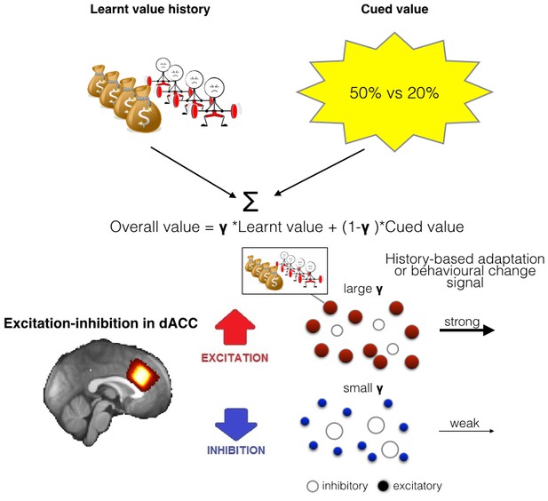
Illustration of the model of integration and use of learnt information and relationship between spectroscopy and brain activity.
(A) People chose between different options by comparing their overall values. The overall value is based on a combination of learnt value (reward and effort magnitudes) and cued value (probabilities). How much they take learnt value, i.e. past reinforcement and effort, into account when making decisions is captured by a single factor, γ. (B) As dACC has previously been linked to both learning about rewards and effort we measured neurotransmitter levels in this region. We propose that the excitation-inhibition balance in dACC affects the use of learnt information relating to both reward and effort in the following way: dACC has a representation of the learnt information, maybe in the form of a model (Karlsson et al., 2012). When there is more overall excitation in this circuit (in red), then dACC representations of value history are more active, ensuring effective distribution of such information to other circuits, ultimately leading to more impact of this factor in behavior. In contrast, when there is relatively more inhibition in dACC, dissemination from dACC is reduced, minimizing the impact of learnt information on other brain areas and on behavior.
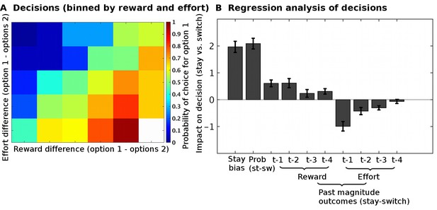
Task validation.
(A) The choices of participants, between the two options, were guided by the reward and effort differences between the options (estimated from a Bayesian learning model): participants were more likely to choose options with higher predicted reward magnitudes and lower predicted effort magnitudes. (B) In a logistic regression analysis, we measured the impact of different factors on choices to either select the same option again as on the previous trial (‘stay’) or to instead select the alternative option (‘switch’). The factors we included were: the reward probabilities (‘prob’) displayed to participants, the reward and effort magnitude outcomes on the past four trials (t-1, t-2, t-3, t-4). This regression showed that participants could use all the relevant information when making their decisions; they used the reward probabilities that were shown on the screen (t(26) = 10.5, p=8*10−11), the past reward magnitudes (ANOVA across all four past trials, main effect: F(1,25) = 53.5, p=1*10−7), and the past effort magnitudes (ANOVA across all four past trials, main effect: F(1,25) = 86.9, p=1*10−9). Data in Figure2_SourceData.xlsx
-
Figure 2—source data 1
This table contains the regression coefficients for individual participants for the analysis shown in Figure 2B.
- https://doi.org/10.7554/eLife.20365.005
-
Figure 2—source data 2
This table relates to Figure 2—figure supplement 1.
It contains data of 270 simulated participants, including the simulated parameters (‘simulated’, ‘s’), the parameters that were estimated from the computational model M1 (‘fitted’, ‘f’) and the regression weights (‘w’) resulting from performing the same behavioral regression as on the real data, see Materials and methods, section ‘task validation’.
- https://doi.org/10.7554/eLife.20365.006
-
Figure 2—source data 3
This table relates to Figure 2—figure supplement 2.
It contains the model fits (Bayesian Information Criterion, BIC) for a non-hierarchical version of all models (models one to six, M1-M6) and the individual parameters for all participants from the hierarchical version of model M1. The individual parameters are shown for a model fitted on behavioral data from both sessions combined (‘both session’, ‘bs’), for a model fitted on data from the MRI session only (‘MRI session’, ‘ms’) and for a model fitted on data from outside the MRI scanner only (‘outside MRI session’, ‘os’).
- https://doi.org/10.7554/eLife.20365.007
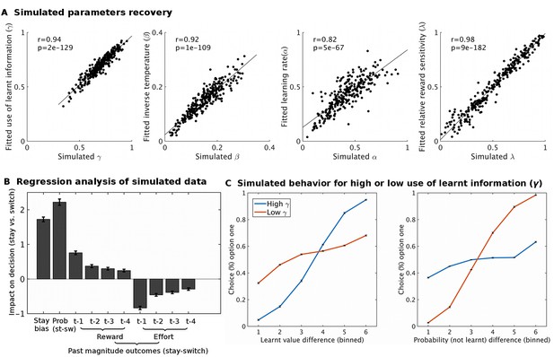
Model simulation and validation.
Using fitted group level parameter estimates for model M1, ten sets of 27 participants (same data set size as real data) were generated. These sets were analyses using the same modeling approach as the real data. Different analyses showed that the behavioral model was appropriate: (A) The model was able to recover parameters well; i.e. the fitted parameter estimates were very similar to the simulated parameters (all p<10−66). (B) A regression analysis, analogous to the one performed on real data (Figure 2B), showed that the simulated data recaptures the patterns of the real data well. (C) To illustrate the expected effect of varying the use of learnt information (γ) to guide behavior we simulated two groups of 270 participants that varied in this parameter (group ‘high γ’ = 0.92; group ‘low γ’ = 0.33). When the learnt information is used a lot (high γ, blue line), the proportion of choices is more influenced by the difference in learnt value (left hand side plot) than by the difference in cued probability (right hand side plot). The opposite pattern is found when the learnt information is used little (low γ, red line). Data in Figure2_SourceData2.xlsx
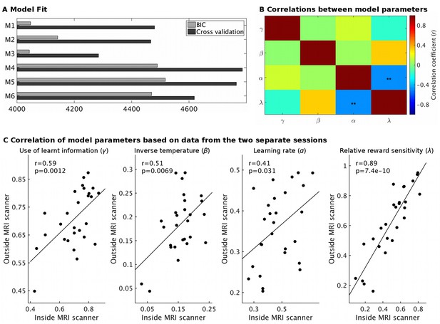
Model fit and parameter stability.
(A) The behavioral models differed in the number of learning rates they employed, either sharing a single learning rate for learning about reward and effort (M1 and M4) or using separate learning rates (M2 and M5) or not using a free learning rate and instead using predictions derived from a Bayesian optimal observer model (M3 and M6). The models also differed in whether reward magnitude and probability were integrated as a weighted linear sum (M1-M3) or whether they were multiplied with each other (M4-M6). Model fit was assessed using either BIC (grey) on a non-hierarchical version of the models or using half-split cross validation (2*negative log likelihood, black, using data from the session only inside or outside the scanner to fit the model and the remaining session as test set) on the hierarchical models. Lower values indicate better fit. On both measures, models using linear integration of magnitude and probability (M1-M3) provided an overwhelmingly better fit, as found previously (Scholl et al., 2014). While the model fit measures do not agree on whether modeling learning with a shared or separate learning rates (α) is best (M1 vs. M2), we note that for the key parameter of interest here, the use of learnt information (γ), we obtain the same value using either model (r = 1.0, p<10−36). We have therefore used the simpler model (M1) throughout. We also note that the excellent model fit for M3 shows that the Bayesian optimal observer model that we used to generate regressors for the fMRI and behavioral regression analysis provides a good fit to the data. (B) Correlations between model parameters derived from M1 (hierarchical version). Importantly, the use of learnt information (γ, top row) did not correlate significantly with any other model parameter (all r < 0.14; all p>0.43). **p<0.01. (C) Model parameter estimates for each participant derived either from the behavior measured inside the MRI scanner or on the next day outside the MRI scanner showed high correlations, in particularly for the use of learnt information (r = 0.59, p=0.0012). This shows that our model-derived measurements have high test-retest reliability. Data in Figure2_SourceData3.xlsx
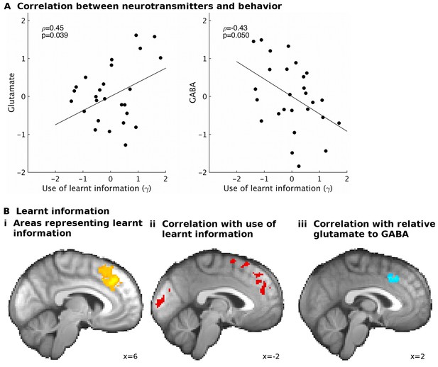
GABA and glutamate predict behavior and neural activity.
(A) Participants with higher concentrations of glutamate (ρ=0.45, p=0.039) and lower concentrations of GABA (ρ=−0.43, p=0.05) in dACC were better able to use the learnt information (parameter γ from computational model) to guide their choices (the graphs illustrate partial correlations, i.e. the plotted values have been adjusted for covariates, see Materials and methods). (Bi) Neural activity in dACC was sensitive to the information to be learnt at the time of the outcome: it showed an inverse outcome value signal, i.e. BOLD activity increased with relative value of the alternative (unchosen minus chosen option, reward minus effort magnitude;yellow, whole-brain cluster-corrected, p=5*10−5, GLM1). (Bii) Individual differences in this neural signal were predictive of individual differences in how well participants could use the learnt information (red, whole-brain cluster-corrected, p=2*10−5, GLM2). (Biii) Individual differences in this neural signal also correlated with relative glutamate and GABA levels (blue, cluster-corrected in spectroscopy ROI, p=0.039, GLM3). See Figure 3—figure supplement 2 for overlaps of these activations with the spectroscopy voxel in sagittal cross-sections. Data for A in Figure3_SourceData1; data for B in Figure3_SourceData2.zip
-
Figure 3—source data 1
This table contains the spectroscopy, brain volume and behavioral parameters used for correlations in Figure 3A.
- https://doi.org/10.7554/eLife.20365.011
-
Figure 3—source data 2
This folder contains the MRI contrast maps, both thresholded (i.e. corrected for multiple comparison using cluster correction) and non-thresholded.
The maps are in NIfTI format and can be opened with freely available data viewers such as FSLView or MRIcron.
- https://doi.org/10.7554/eLife.20365.012
-
Figure 3—source data 3
This folder relates to Figure 3—figure supplement 3.
It contains non-thresholded contrast maps showing the relationship between Glu-GABA and brain activity to information to be learnt, using different corrections of spectroscopy measurements for partial brain volumes (Figure 3—figure supplement 3i). Maps are in NIfTI format.
- https://doi.org/10.7554/eLife.20365.013
-
Figure 3—source data 4
This table relates to Figure 3—figure supplement 3.
It contains the brain-volume corrected spectroscopy measurements (brain volume corrections B-D labeled as in figure) and behavioral parameters used for correlations in Figure 3—figure supplement 3ii.
- https://doi.org/10.7554/eLife.20365.014
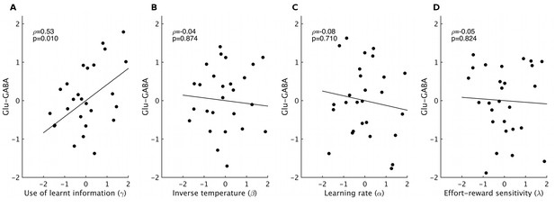
Correlations between spectroscopy measurements and other behavioral parameters.
Based on previous research, we had strong predictions that spectroscopy measures in dACC should relate to the use of learnt information. Nevertheless, to check the specificity of our effect, we also correlated spectroscopy measures from dACC with the other model parameters that we obtained. We found high specificity: while relative glutamate minus GABA levels correlated with the use of learnt information (A, non-parametric partial correlation, ρ=0.53, p=0.010), they did not correlate with either inverse temperature (B), learning rate (C) or relative sensitivity to reward compared to effort (D) (non-parametric partial correlations, all p>0.7). The significance level for Bonferroni correction for four t-tests is 0.0125.
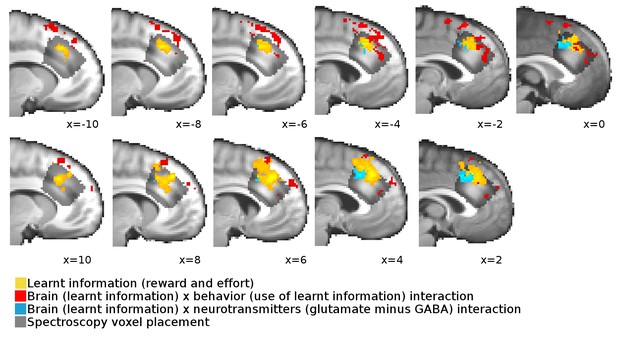
Overlap between neural signals and spectroscopy voxel placements.
Cross-sections from x=−10 to x = 10 through the brain show the overlap, extent and spatial pattern of the activations reported in Figure 3B in the main text and the placement of the spectroscopy voxel.
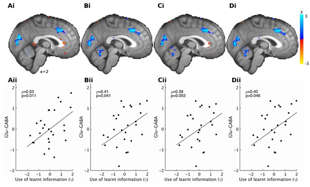
Different brain volume normalizations for spectroscopy.
Previous papers have corrected spectroscopy measurements for partial brain volume in the spectroscopy voxel using different procedures (Jocham et al., 2012; Stagg et al., 2009; Terhune et al., 2014). (i) Using these different corrections, we find very similar results for correlations between relative glutamate minus GABA and neural activity encoding the value to be learnt (reward minus effort). Results are shown at reduced voxel-wise threshold of p<0.05 for illustration; blue areas show increased representation of information to be learnt with the glutamate minus GABA contrast, red areas show decreased representation of information to be learnt with glutamate minus GABA contrast. (ii) We also find that the correlations between relative glutamate minus GABA and the behavioral measure of the use of learnt information (γ) are very similar for different ways of correcting for partial brain volumes. The corrections used were: (A) including relative grey and white matter and total tissue as separate covariates (same as reported in main text), (B) correcting glutamate and GABA by: glutamate (GABA) divided by creatine divided by relative grey matter, (C) correcting glutamate and GABA by: glutamate (GABA) divided by creatine divided by relative grey + white matter, (D) correcting glutamate and GABA by dividing by relative grey matter and correcting creatine by dividing by relative grey + white matter, before dividing corrected glutamate (GABA) by corrected creatine. Data in Figure3_SourceData3.zip and Figure3_SourceData4.xlsx
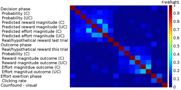
Correlations between regressors in GLM1.
We used three boxcar regressors for the three phases of the task: Decision phase (from the beginning of the trial until participants made a choice), Outcome phase (from the appearance of the chosen outcome until the chosen and the unchosen outcomes disappeared from the screen) and lastly the Effort exertion phase (from the appearance of the first effort target until participants had removed the last target). We included the following parametric regressors in the decision phase: the reward probabilities that were shown on the screen, the predicted reward and effort magnitudes (derived from a Bayesian learning model; we note that the regressors for reward and effort magnitudes obtained in this way correlated very strongly (r>0.99) with those obtained from the fitted reinforcement learning model). These regressors were included separately for the chosen and unchosen option. We also included a regressor indicating whether reward had been real or hypothetical on the last trial [because rewards were probabilistic they were only delivered on some trials (real reward trials) while on other trials participants were just informed what the reward would have been had it been delivered (hypothetical reward)]. In the outcome phase, we included the following parametric regressors: whether the reward delivered for the chosen option was real or hypothetical, the reward probability for the chosen option and the reward and effort magnitude outcomes for the chosen and the unchosen options. The onset of all regressors for the chosen option was time-locked to the onset of the outcome phase; the onset and duration of the regressors for the unchosen option were timelocked to their display. In the effort exertion phase, we included the clicking rate as a parametric regressor. Finally, we included, as confound regressors, six movement regressors and a regressor indexing when additional visual stimuli were presented to warn participants that they had not clicked the targets on time and that the halfway point of the experiment had been reached (‘Confound – visual’). Correlations between the different regressors are indicated as a heat map; no correlations (r-values) exceeded 0.33.
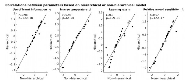
Correlations between model parameters derived using either a hierarchical (y-axis) or non-hierarchical (x-axis) model fitting approach.
https://doi.org/10.7554/eLife.20365.020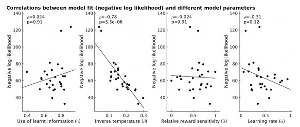
The fit of the model for each participant (measured as negative log likelihood, y-axis) strongly correlates with the estimate of inverse temperature (β) from the model (ρ=-0.78, p=3.5x10⁻⁶).
However it does not correlate with other model parameters (all p>0.12).
Tables
(A) Several areas carried a signal for learnt information (relative reward outcome minus relative effort outcome) as an inverse outcome value signal, in other words a signal related to the value of the alternative choice compared to the value of the action actually taken. (B) Other areas signaled outcomes to be learnt as the value of the action actually taken relative to the value of the alternative action. (C) Areas in which individual differences in the strength of the neural signal for the learnt information correlated with the behavioral use of the learnt information. All results are cluster-corrected at whole-brain level (z > 2.3, p<0.05, with actual p-value and number of voxels in the cluster indicated in the table). Region labels were obtained using atlases in FSL: 1(Neubert et al., 2015), 2(Mars et al., 2011), 3(Sallet et al., 2013), 4(Mori et al., 2005).
A) Learnt information (inverse value signal) | ||||||
|---|---|---|---|---|---|---|
x | y | z | z-score | Voxels | p-value | |
dACC (area 8m, anterior rostro-cingulate zone1) | 6 | 32 | 36 | 3.62 | 821 | 5*10−5 |
Parietal (IPL-D, IPL-C2), left | −52 | −58 | 42 | 3.68 | 855 | 3*10−5 |
Parietal (IPL-C, IPL-D2), right | 52 | −46 | 42 | 3.98 | 753 | 1*10−4 |
Dorsolateral prefrontal cortex (area 9/46 V3), right | 40 | 22 | 38 | 3.61 | 840 | 4*10−5 |
Cerebellum | −10 | −80 | −26 | 4.19 | 454 | 6*10−3 |
Lateral frontal pole1, right | 32 | 54 | 6 | 3.21 | 360 | 0.02 |
B) Learnt information (outcome value signal) | ||||||
Temporal cortex, extending to parietal opercular cortex, left | −36 | −32 | 16 | 3.49 | 1371 | 1*10−7 |
Temporal cortex, extending to parietal opercular cortex, right | 50 | −28 | 26 | 3.23 | 458 | 5*10−3 |
C) Brain behavior interaction for learnt information | ||||||
Midcingulate cortex (posterior rostro-cingulate zone1) | 2 | −4 | 54 | 3.12 | 719 | 2*10−4 |
Pre-SMA extending into dACC and area 8 m1 | −14 | 24 | 58 | 3.44 | 771 | 2*10−5 |
Occipital lobe | −12 | −84 | 4 | 3.22 | 488 | 0.001 |
White matter (corticospinal tract4) | −18 | −14 | 32 | 3.4 | 431 | 0.003 |
Precentral gyrus, right | 40 | −14 | 52 | 3.28 | 311 | 0.02 |


