Multivariate cross-frequency coupling via generalized eigendecomposition
- Donders Center for Neuroscience, Radboud University Nijmegen Medical Centre, Radboud University, Netherlands
Figures
Figure 1 with 3 supplements
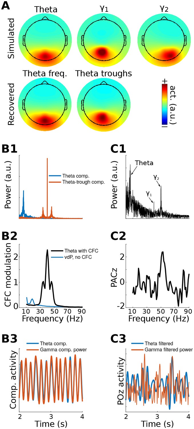
gedCFC Method 1 applied to simulated data.
Data were generated in three dipoles in the brain and projected to the scalp (top row of (A)) along with correlated 1/f noise at 2,001 other dipoles. The theta component (~6 Hz) was recovered by GED (bottom row of (A)). The 40 Hz component was recovered using gedCFC on broadband data. (B) shows the power spectrum of the theta and theta-trough components (B1), the strength of CFC (B2), and illustrative time courses (B3). The blue line in (B2) corresponds to a van der Pol oscillator (vdP), which causes spurious high-frequency CFC in traditional analyses. (C1) shows the power spectrum of electrode POz, which is the spatial maximum of the EEG data power. Note that the 50 Hz gamma (γ2) has larger power than the 40 Hz (γ1). (C2) illustrates that traditional phase-amplitude coupling with permutation testing (PACz) applied to channel POz failed to recover the simulated CFC patterns. (C3) shows the poor reconstruction of the dynamics when using data from POz (compare with (B3)).
Figure 1—figure supplement 1
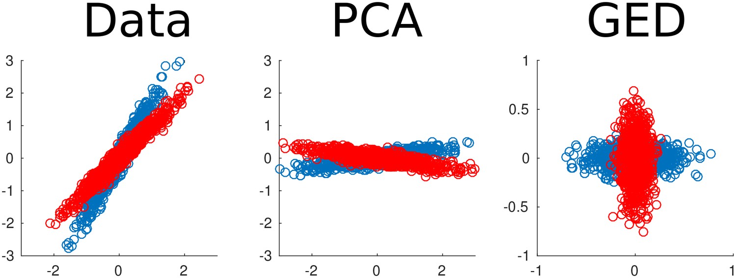
Two-dimensional example of using generalized eigendecomposition (GED) to separate sources.
Two data streams were created (red and blue dots). Principal components analysis (PCA) rotated the entire data set, while GED separated the two components. This was done using the equation = RWΛ, where S and R were covariance matrices from the red and blue data streams. This illustration is modeled after Figure 6 of Blankertz et al. (2008).
Figure 1—figure supplement 2
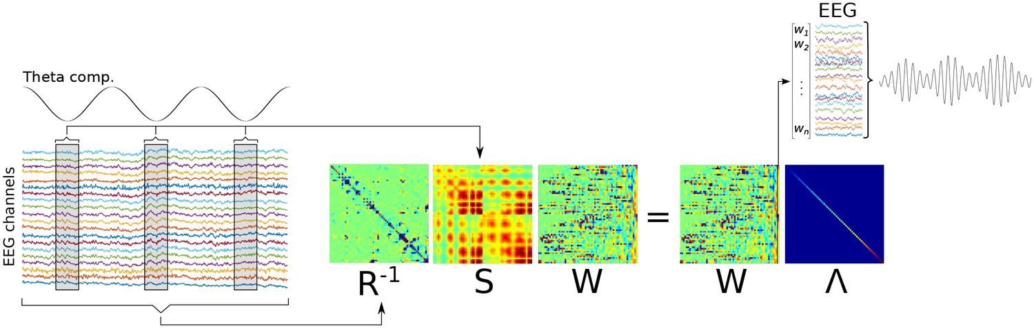
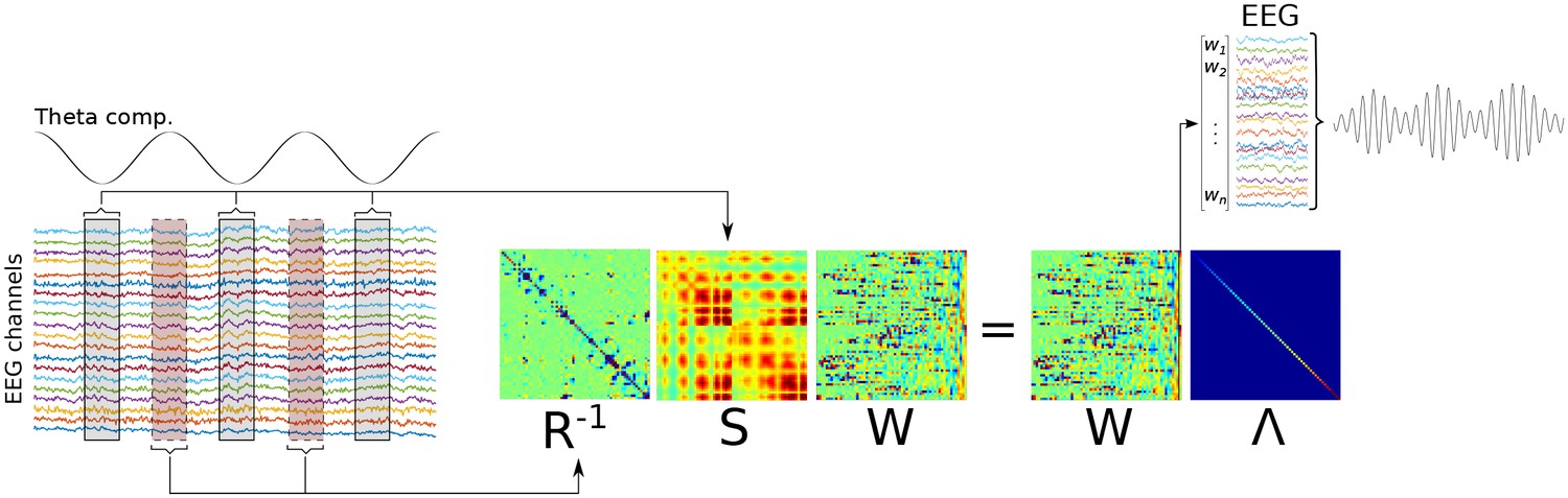
Graphical overview of Method 1.
A low-frequency component is identified (‘Theta comp.’), and covariance matrices are computed on the basis of the multichannel data surrounding each trough, and using all data (respectively, S and R matrices). A generalized eigendecomposition of these matrices provides a set of eigenvectors (matrix W). The eigenvector with the largest eigenvalue (diagonal of matrix Λ) is used as weights to combine data from all channels linearly, which produces the component that best differentiates trough-related from non-trough-related activity.
Figure 1—figure supplement 3
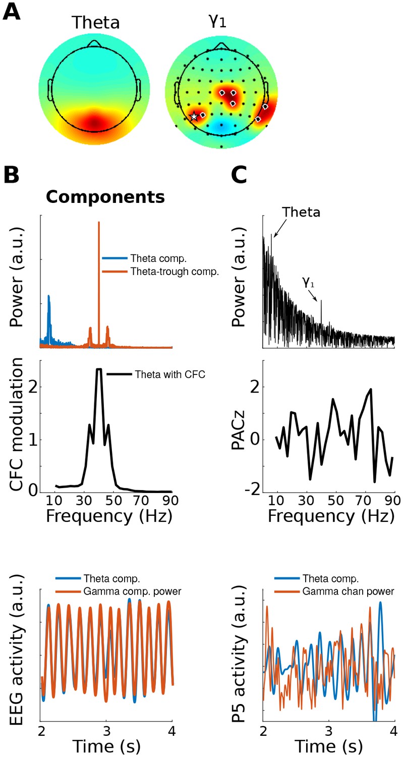
This figure is similar to Figure 1, except that the gamma modulation was simulated in a collection of electrodes instead of in a dipole projected to the scalp.
This shows that gedCFC makes no assumptions regarding spatial smoothness or autocorrelation. The electrodes with black/white circles show where the gamma bursts were simulated, and the electrode with the white star shows the electrode selected for analyses in (C).
Figure 2

Method 1 applied to empirical MEG resting-state data.
An alpha component was computed using GED; its topographical projection and power spectrum are shown in (A1) and (A2). Covariance matrices from broadband data surrounding high-power alpha peaks were computed, and were entered into gedCFC using a covariance matrix from the broadband signal from the entire time series as reference. The first three components (topographical projections and projections onto the cortical surface in (B1)) along with their time-frequency power spectra locked to alpha peaks (B2) are shown.
Figure 3 with 1 supplement

Method 2 applied to simulated data.
Gamma power (40 and 45 Hz) in two brain dipoles was modulated by a theta wave from a third dipole. Activity from these three dipoles was projected, along with correlated 1/f noise from 2,001 other dipoles, to 64 scalp EEG channels (top row of (A) shows the signal-dipole projections). gedCFC was able to recover these three components ((A), bottom row) by comparing broadband covariance matrices between theta peaks and troughs. (B) shows the time-frequency power spectra of the components time series time-locked to theta peaks and theta troughs. (C) shows power spectra of the three component time series. For comparison, the power spectrum from POz (the channel with maximum power) is shown. (D) shows CFC modulation defined as the average peak-trough distances per frequency. (E) shows a 2 s snippet of data from the theta component and the power time courses from the theta-peak and theta-trough components. The lower panel shows data from POz bandpass filtered around theta, 40 Hz, and 45 Hz. Note that the continuous gamma power time series closely matched the theta wave from which they were simulated, although the covariance matrices were taken only from peaks and troughs.
Figure 3—figure supplement 1
This figure shows a graphical overview of Method 2.
It is similar to Method 1 (see Figure 1—figure supplement 2) except that the R matrix is computed from data surrounding low-frequency peaks instead of the entire time series.
Figure 4
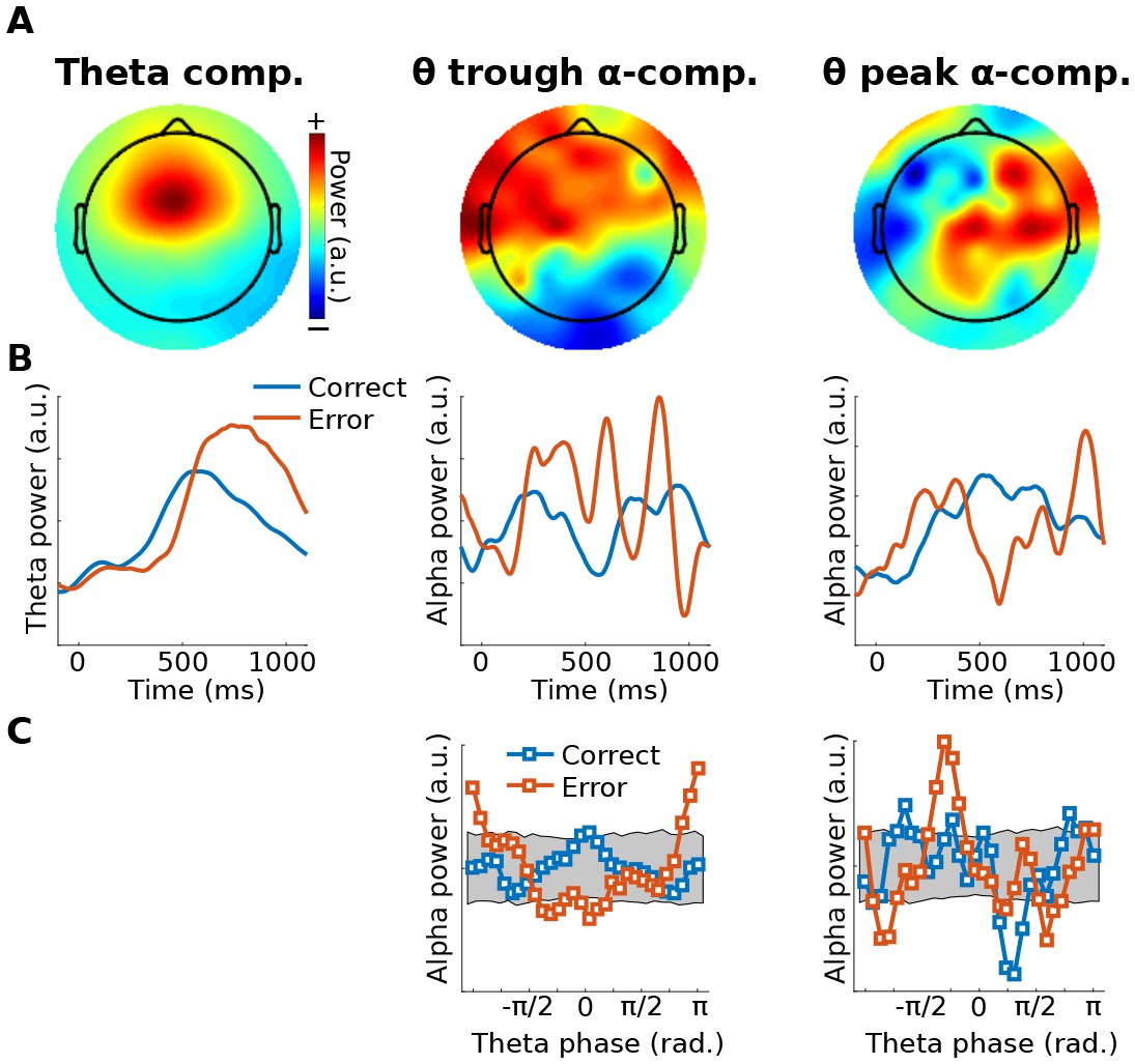
Illustration of Method 2 applied to real EEG data.
The human volunteer (one subject selected from Cohen and van Gaal (2013)) performed a speeded reaction time task in which response errors frequently occurred. (A) shows topographical projections of the three components (theta power, theta trough, theta peak). (B) shows power time courses relative to stimulus onset (time = 0) from those components, separately for correct and error trials (power was extracted via the filter-Hilbert method). (C) shows how alpha power in the two alpha components fluctuated as a function of theta phase. Note that gedCFC was based on data from all trials pooled; the two experiment conditions were separated only when plotting. The gray bars in (C) show 95% confidence intervals based on 1,000 permutations in which the assignment between theta phase and alpha power was shuffled.
Figure 5 with 1 supplement
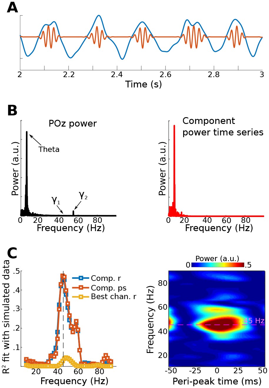
Results from simulation for Method 3.
Data were simulated in the same dipoles used in Method 1. (A) shows an example of the dipole time series, illustrating the theta wave and the gamma modulation (scaled for visibility). Power time series were extracted from all channels, and the low-frequency time series was used as a bias filter against the multichannel power time series matrix. (B) shows the power spectrum from channel POz (left panel). Note the absence of a prominent 45 Hz peak. The right panel shows the power spectrum of the 45 Hz power time series from the gedCFC component. The peak at 6 Hz reflects the modulation of 45 Hz power by the theta rhythm. (C) shows the fit (correlation or phase synchronization) between the gedCFC component per frequency and the simulated power time series. For comparison, the correlation result was also performed at channel POz. The right panel shows the time-frequency power spectrum locked to theta peaks.
Figure 5—figure supplement 1
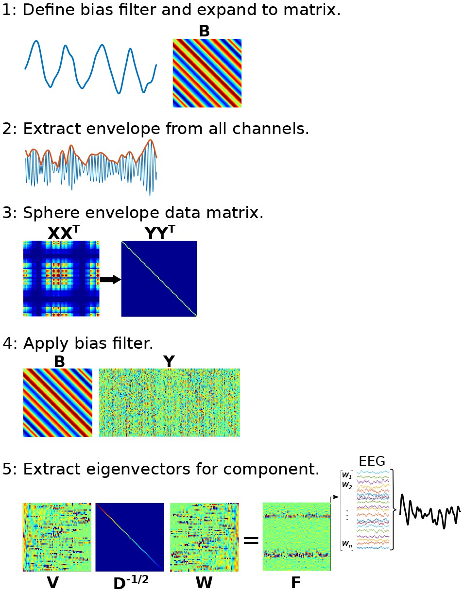
Graphical overview of the procedure for applying joint decorrelation adapted to Method 3.
(1) The bias filter is a low-frequency dynamic to be used as the time series ‘seed’ for identifying CFC. It is expanded to a matrix using the Toeplitz operation. (2) The analytic envelope from each data channel is extracted and mean-centered to form a new data matrix, X. (3) The data are sphered to remove intrinsic covariance patterns, forming a new data matrix Y; sphering turns the covariance matrix into a diagonal matrix. (4) The bias filter multiplies Y, which computes the dot product between temporally shifted versions of the bias filter and the sphered data. (5) The covariance matrix of BY has eigenvectors W that rotate the eigenspace of X (its eigenvectors are in V and eigenvalues are in D) as matrix F. The largest-valued eigenvector in F defines the multivariate component that best matches the bias filter.
Figure 6
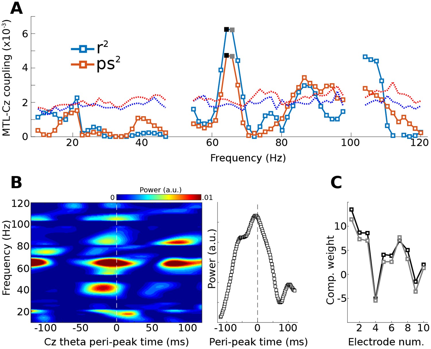
Method 3 applied to empirical data from a human epilepsy patient, with ten channels in the medial temporal lobe (MTL) and Cz, a scalp electrode that measures midline frontal activity.
Covariance matrices of MTL channels were created locked to peaks from Cz filtered at 4 Hz. (A) shows the coupling strengths, measured both as correlations (r) and as phase synchronization (ps) over a range of frequencies (notch-filtered data at 50 Hz and 100 Hz are omitted). Correlation values were squared to avoid sign issues, and phase synchronization values were squared for comparability. The dotted lines indicate the 99% confidence intervals based on 1,000 permuted shufflings. (B) shows the time-frequency power spectrum of the MTL component time-locked to Cz theta peaks. The right plot shows the time course of activity averaged around 65 Hz (frequencies selected based on visual inspection of (A). (C) illustrates the component weighting across the ten MTL electrodes from two neighboring frequencies (see black and gray filled squares in (A); smaller numbers are anterior).
Figure 7
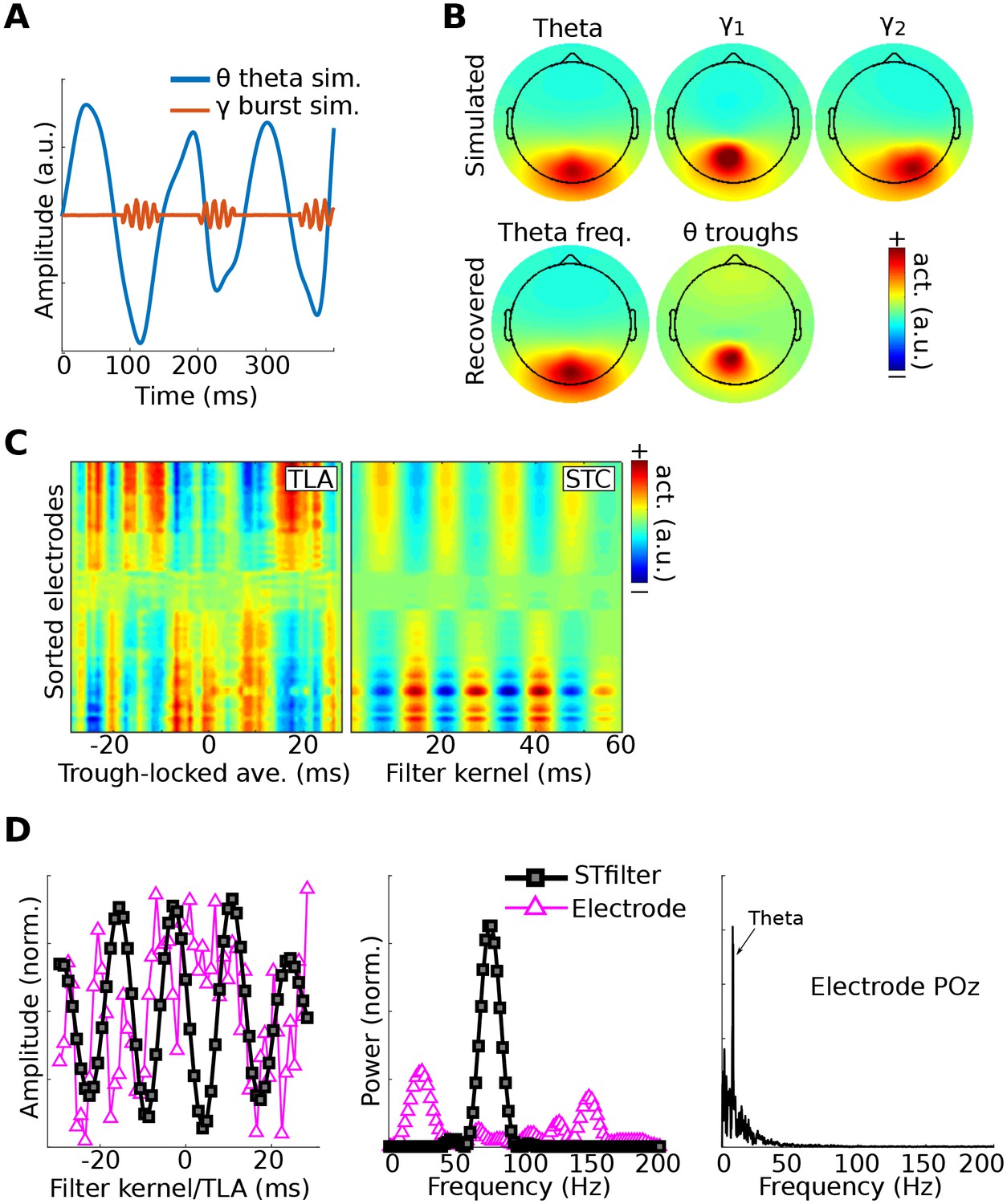
Method 4 applied to simulated EEG data.
Bursts of 75 Hz gamma in one dipole were locked to theta troughs in a different dipole (A). Activity in these two dipoles, along with a ‘distractor’ gamma signal at 50 Hz and correlated 1/f noise at all other dipoles, was projected to scalp EEG channels. (B) shows the dipole projections and their reconstructions from gedCFC on delay-embedded matrices. (C) shows the trough-locked average (TLA) over time for all electrodes (electrodes are sorted according to spatial location, with anterior electrodes on top and posterior electrodes on the bottom) on the left and the spatiotemporal component (STC) extracted via gedCFC on the right. (D) shows the time series of the filter kernel from electrode POz (left), the filter kernel power spectrum (middle), and the power spectrum of POz activity (right; note the absence of a pronounced peak at 75 Hz). Even with only minimal noise, the non-phase-locked nature of the gamma burst prevented the TLA from revealing any meaningful relationship (phase-locking does not affect the single-trial covariance matrices). Amplitudes are normalized to facilitate direct comparisons.
Figure 8
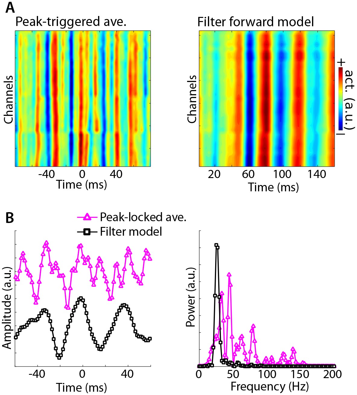
Illustration of Method 4 applied to empirical data from rodent hippocampus.
GED was used to identify a theta component (peak frequency 8 Hz), and peak times were identified. (A) illustrates the peak-triggered LFP trace over 32 channels (high-pass filtered at 20 Hz), and the forward model of the first gedCFC component. (B) illustrates the peak-locked average and the component model, averaged over all channels, in the time domain (left panel) and in the frequency domain (right panel). Amplitudes were scaled and y-axis-shifted for comparability.
Figure 9
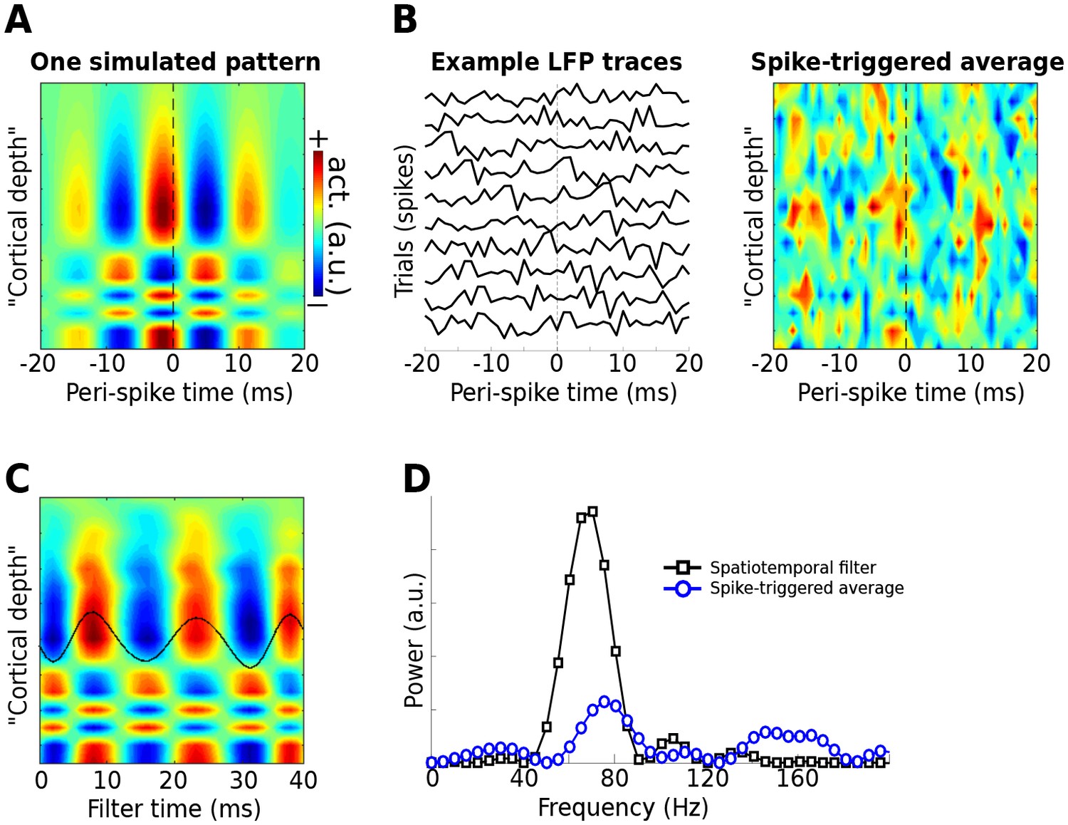
Use of the gedCFC framework for detecting spike-field coherence in multichannel data.
LFPs were simulated in 16 channels, modeled after a silicon probe often used to measure cortical laminar activity. Forty random spike times were generated, and complex spatiotemporal patterns were time-locked to each spike time. (A) illustrates the basic pattern, which was phase-randomized on each spike. (B) illustrates a few single-spike LFP traces from one channel, and the spike-triggered average over time and space (compare with the template in (A)). (C) shows the forward model from the largest gedCFC component reshaped to a 2D matrix. (D) shows the power spectrum of the component and the spike-triggered average (power spectra averaged across channels).
Figure 10 with 1 supplement
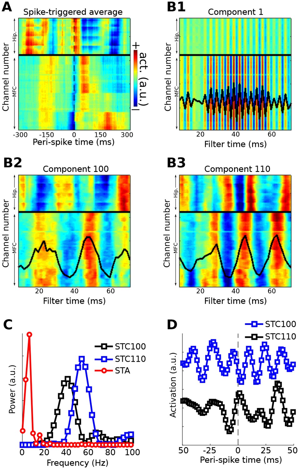
Method 5 applied to rodent hippocampal-prefrontal single-cell and LFP recordings.
(A) shows the spike-triggered average across all channels (MFC = medial frontal cortex; Hip. = hippocampus). (B) illustrates the forward models of several gedCFC components. The first few components captured the spike artifact, as shown in (B1). Later components reflected different aspects of physiological activity, two of which are illustrated here ((B2) and (B3)). The power spectra of the spike-triggered average and the two physiological components are shown in (C) (the component spectra have the same y-axis scale; the spike-triggered average was scaled down for comparability; STC = spatiotemporal component). (D) shows the spike-triggered average of the two components (shifted on the y-axis for comparability). Note that the components are temporally asymmetric and nonsinusoidal; their waveform shapes are defined empirically without imposition of a sinusoidal filter.
Figure 10—figure supplement 1
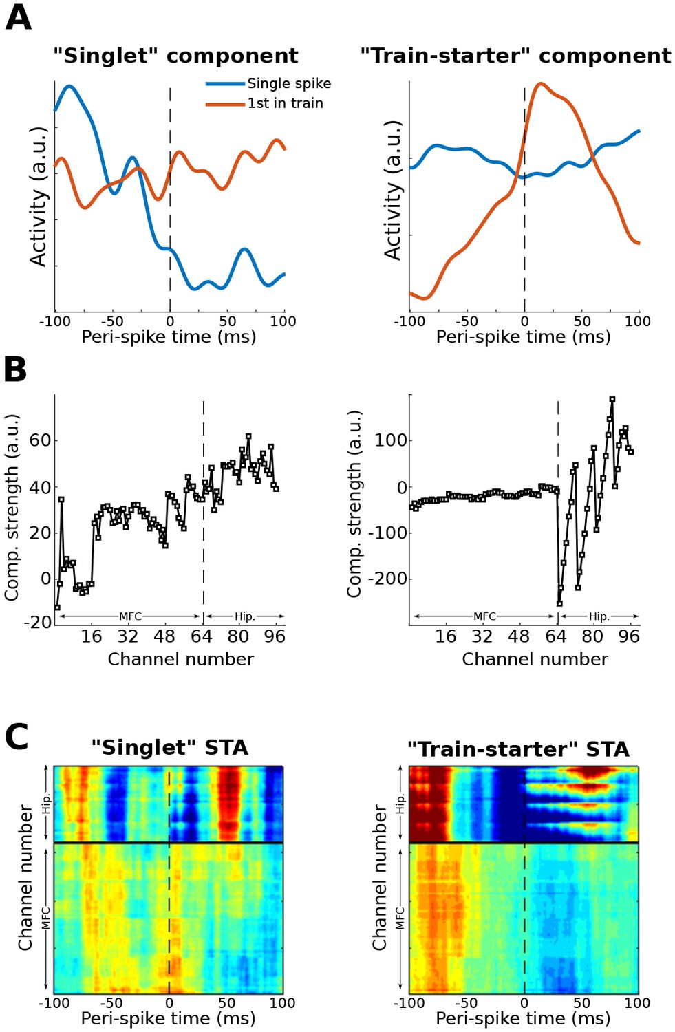
This figure shows another possible application of the gedCFC framework for multivariate spike-field coherence, using the same dataset as used in Figure 10.
Action potentials from a single neuron (different from the one used in Figure 10) in the prefrontal cortex were categorized as ‘singlets’ (no action potentials 100 ms earlier or 100 ms later; N = 58) or as ‘train-starters’ (no action potentials 100 ms earlier, and at least one action potential within 20 ms after; N = 151). LFP covariance matrices were then formed around these two action potential categories and compared using Method 2. The component with the largest and smallest eigenvalues were extracted and treated as ‘singlet’ and ‘train-starter’ components. This figure shows the time courses of those components relative to the spikes, as well as the spike-triggered average LFP traces (STA). The ‘train-starter’ component was dominated by hippocampal activity. The jagged appearance of the weights is consistent with the electrode layout, which had eight electrodes per shank and four shanks.
Tables
Table 1
Overview of methods.
Description | Analysis goal | Key assumption | |
|---|---|---|---|
Method 1 | S defined by peri-LF-peak; R defined by all data | Identify a single phase-amplitude coupled network | One HF network with power proportional to LF phase |
Method 2 | S defined by peri-LF-peak; R defined by peri-LF-trough | Identify two networks that alternate according to LF phase. | Two different HF networks that have power peaks at different LF phases |
Method 3 | LF activity bias-filters sphered data | Use (possibly nonstationary) LF waveform shape to identify a HF component. | Well-defined LF waveform |
Method 4 | Delay-embedded matrix, S and R defined as in Methods 1 or 2 | Empirically determine a CFC-related spatiotemporal filter | Appropriate delay-embedded order |
Method 5 | Similar to Method 4 but data are taken peri-action potential | Empirically determine a spatiotemporal LFP filter surrounding action potentials | Sufficient delay-embedding order; one peri-spike network |
-
Notes. LF = low frequency; HF = high frequency. All methods make the assumption that the spatiotemporal characteristics of the HF activity are stable over repeated time windows from which covariance matrices are computed.
Download links
A two-part list of links to download the article, or parts of the article, in various formats.
Downloads (link to download the article as PDF)
Open citations (links to open the citations from this article in various online reference manager services)
Cite this article (links to download the citations from this article in formats compatible with various reference manager tools)
Multivariate cross-frequency coupling via generalized eigendecomposition
eLife 6:e21792.
https://doi.org/10.7554/eLife.21792


