Opposite initialization to novel cues in dopamine signaling in ventral and posterior striatum in mice
- Harvard University, United States
Figures
Figure 1 with 4 supplements
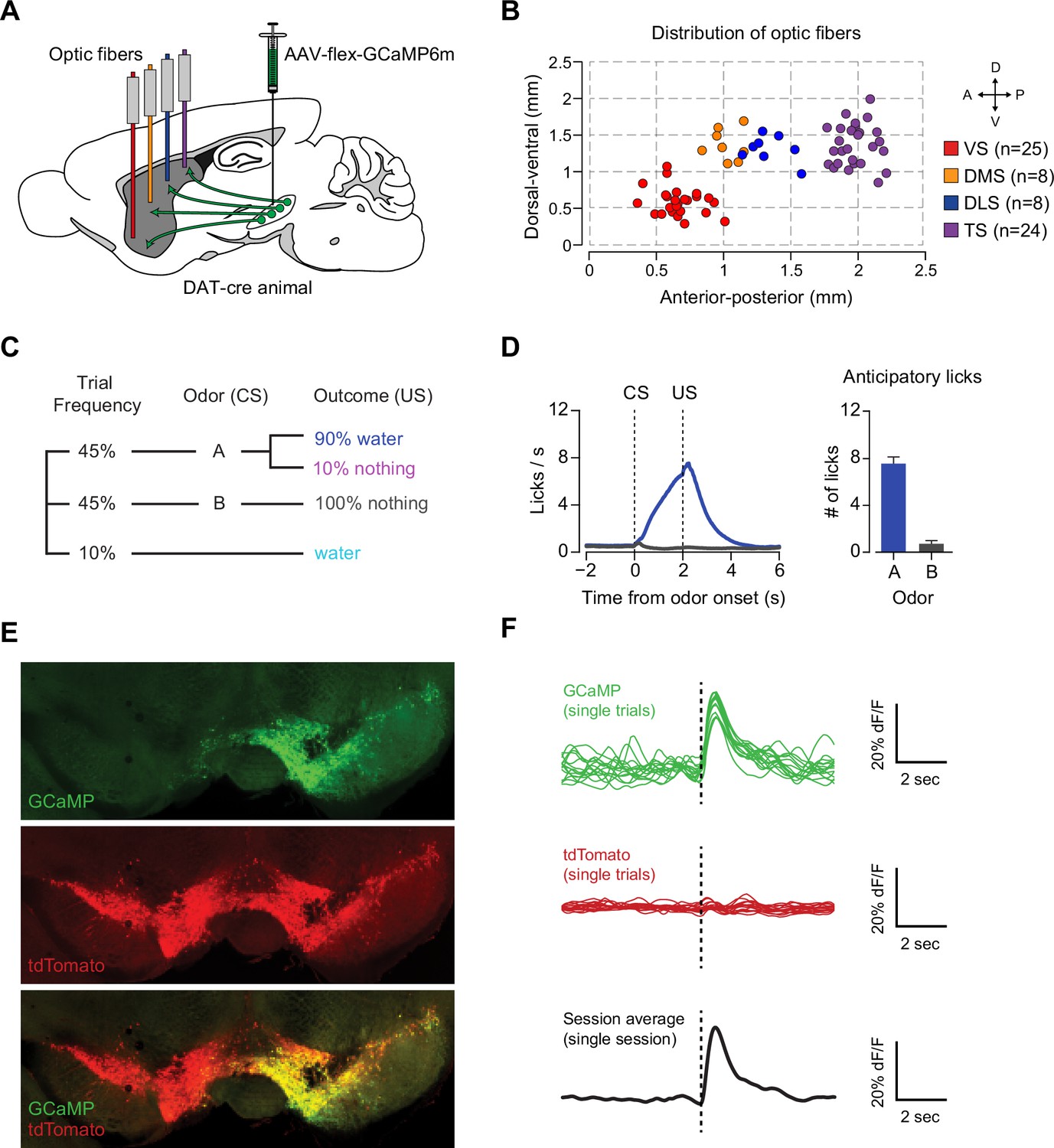
Recording dopamine activity across the striatum using fiber fluorometry.
(A) Schematic of GCaMP virus injection and optic fiber implantation sites. Detailed schematic of recording setup is shown in Figure 1—figure supplement 1. Sample raw data are shown in Figure 1—figure supplement 2. (B) Distribution of optic fibers (sagittal max-projection) used for recording labeled red (VS), orange (DMS), blue (DLS), and purple (TS) with dotted lines denoting ½ mm increments. Coronal sections are shown in Figure 1—figure supplement 3. (C) Schematic of the basic trial structure. An odor cue (CS) (1 s duration) is followed by an outcome (US) or no outcome after 1 s delay, followed by a random inter-trial interval (ITI) of 6–12 s. At a low frequency, unexpected outcomes are also delivered. (D) Licking in response to odors predicting reward (blue) or nothing (grey). Odor onset is t = 0 and water delivery time is t = 2, so anticipatory licking occurs between t = 0 and t = 2 (quantified on the right). (E) An example of GCaMP virus infection. Green indicates AAV-flex-GCaMP6m infection (top), red indicates genetically encoded tdTomato in DAT-cre-expressing neurons (middle), and the bottom panel is an overlay of the two signals. Labeled axons in the striatum are shown in Figure 1—figure supplement 4. (F) Example single trial responses to unpredicted water from GCaMP (top) and tdTomato (middle) from a single session in a mouse with a fiber implanted in VS. The average GCaMP signal across trials in that session are plotted in the bottom panel.
Figure 1—figure supplement 1
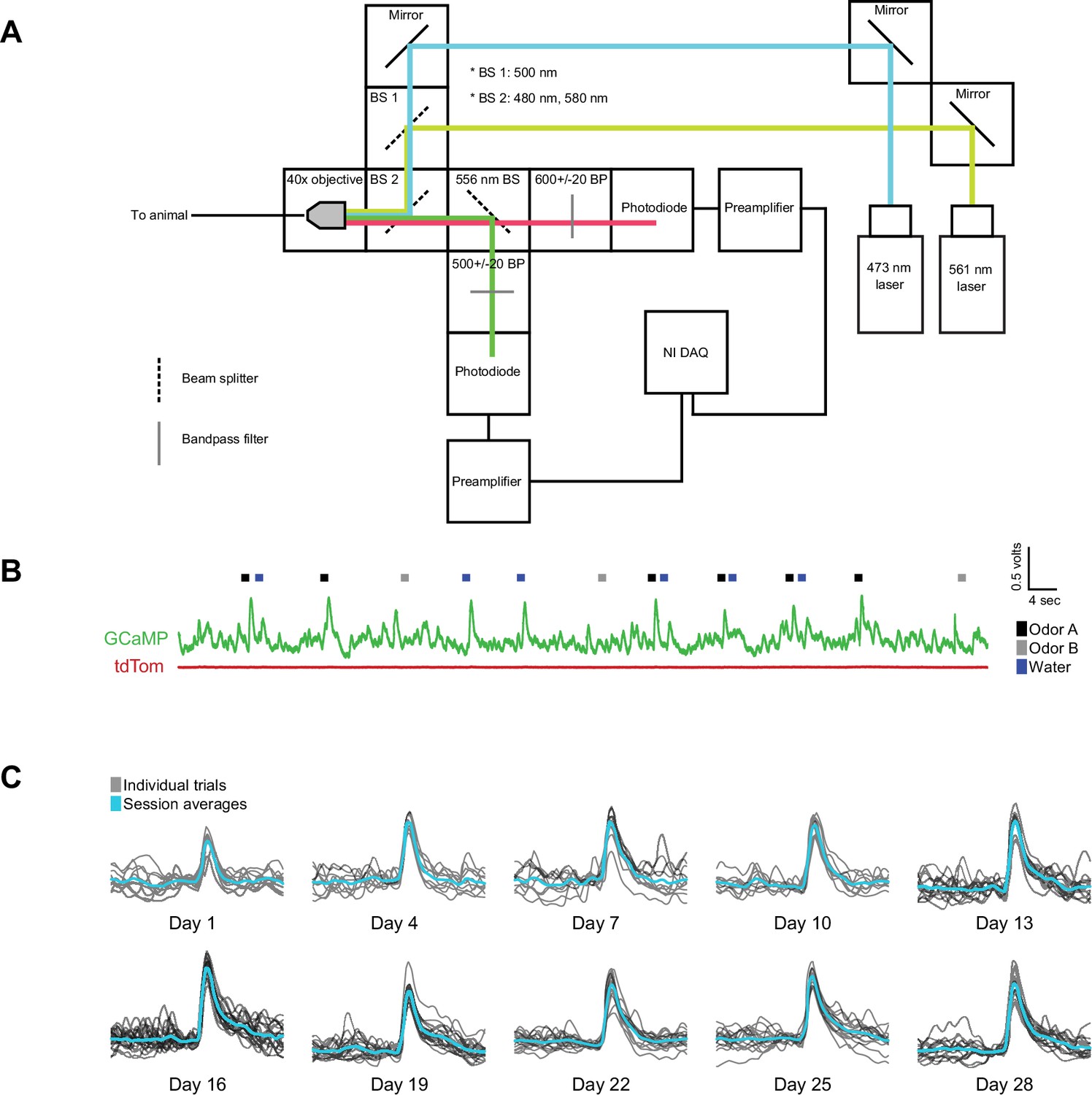
GCaMP6m recording and example traces.
(A) Schematic of recording setup using 473 nm and 561 nm lasers to deliver light, and ultimately a 500 ± 20 nm bandpass filter to collect GCaMP signal and a 600 ± 20 nm bandpass filter to collect tdTomato signal. (B) Example raw voltage traces from each pre-amplifier are shown in green and red. The green trace corresponds to 480–520 nm light and the red trace corresponds to 580–620 nm light. Water delivery times are plotted (blue), along with reward-predicting odor (black) and nothing-predicting odor (grey) delivery times. (C) An example of the individual (grey) and average (blue) unpredicted water responses from a single animal over the course of a month of recording every fourth day are plotted after calculating dF/F.
Figure 1—figure supplement 2
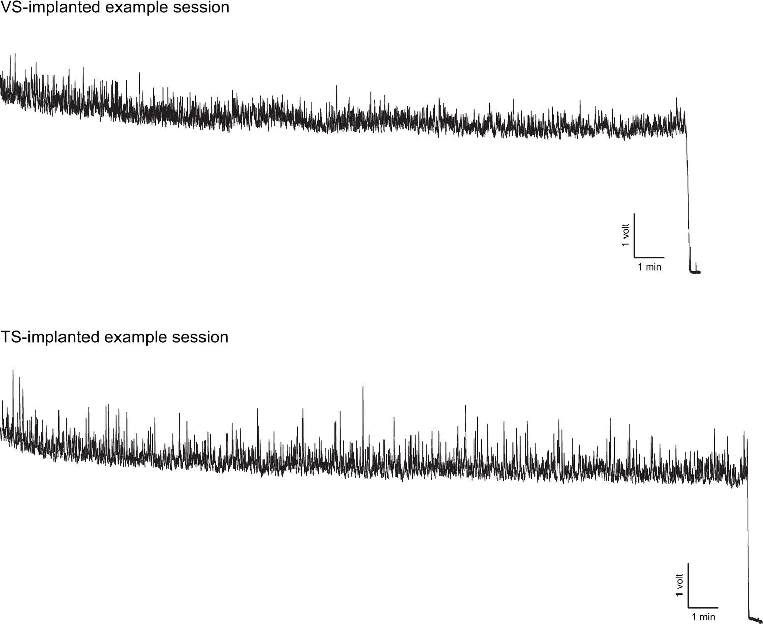
Example recording sessions.
Examples of complete recording sessions from a VS-implanted fiber (top) and TS-implanted fiber (bottom). The signal is the raw voltage continuously measured from the pre-amplifier. Scale bars indicate 1 volt and 1 min. In these sample recording sessions, the excitation laser was on continuously for ~25 min and then turned off (traces dip sharply at the point of laser-off).
Figure 1—figure supplement 3
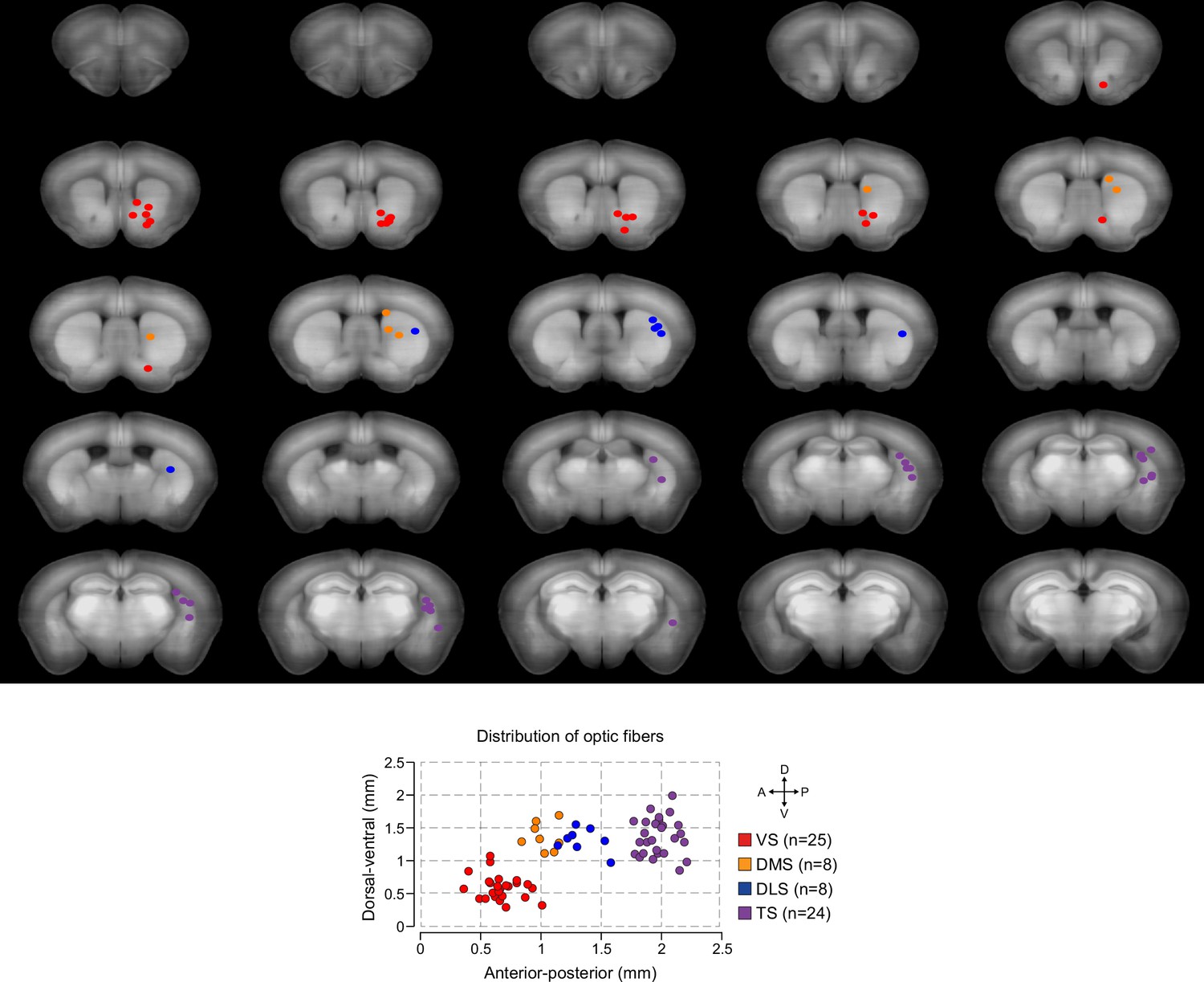
Distribution of recording fibers.
Distribution of recording fibers in VS (red), DMS (orange), DLS (blue), and TS (purple). Each coronal image represents an optical slice that is 100 µm thick, and the fibers that fall within that range are plotted. After image registration, fiber positions were manually identified (see Materials and methods, Figure 7—figure supplement 2). Below, the summary panel from Figure 1B is duplicated.
Figure 1—figure supplement 4
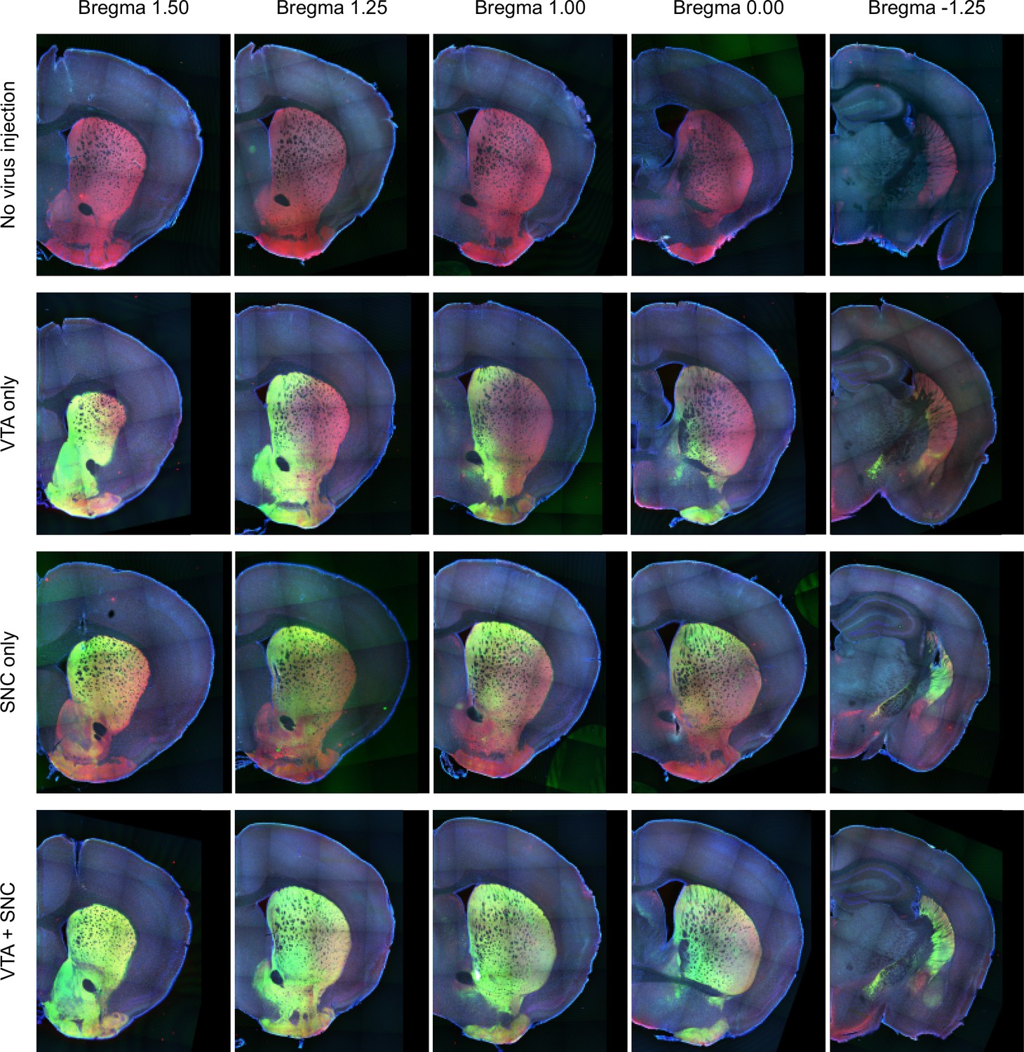
Midbrain dopamine axon distribution in the striatum.
The distribution of dopamine axons from anterior (left) to posterior (right) striatum. Red indicates genetically encoded tdTomato in the axons of DAT+ neurons and green indicates virally encoded GCaMP in the axons of DAT+ neurons. Top row: a mouse expressing tdTomato in dopamine neurons, with no GCaMP virus injection. Second row: GCaMP infection in the VTA only, resulting in stronger labeling of VS axons than TS axons. Third row: GCaMP infection in the SNC only, resulting in stronger labeling of TS axons than VS axons. Bottom row: GCaMP infection in the VTA and SNC, leading to labeling of dopamine axons throughout the striatum.
Figure 2 with 4 supplements
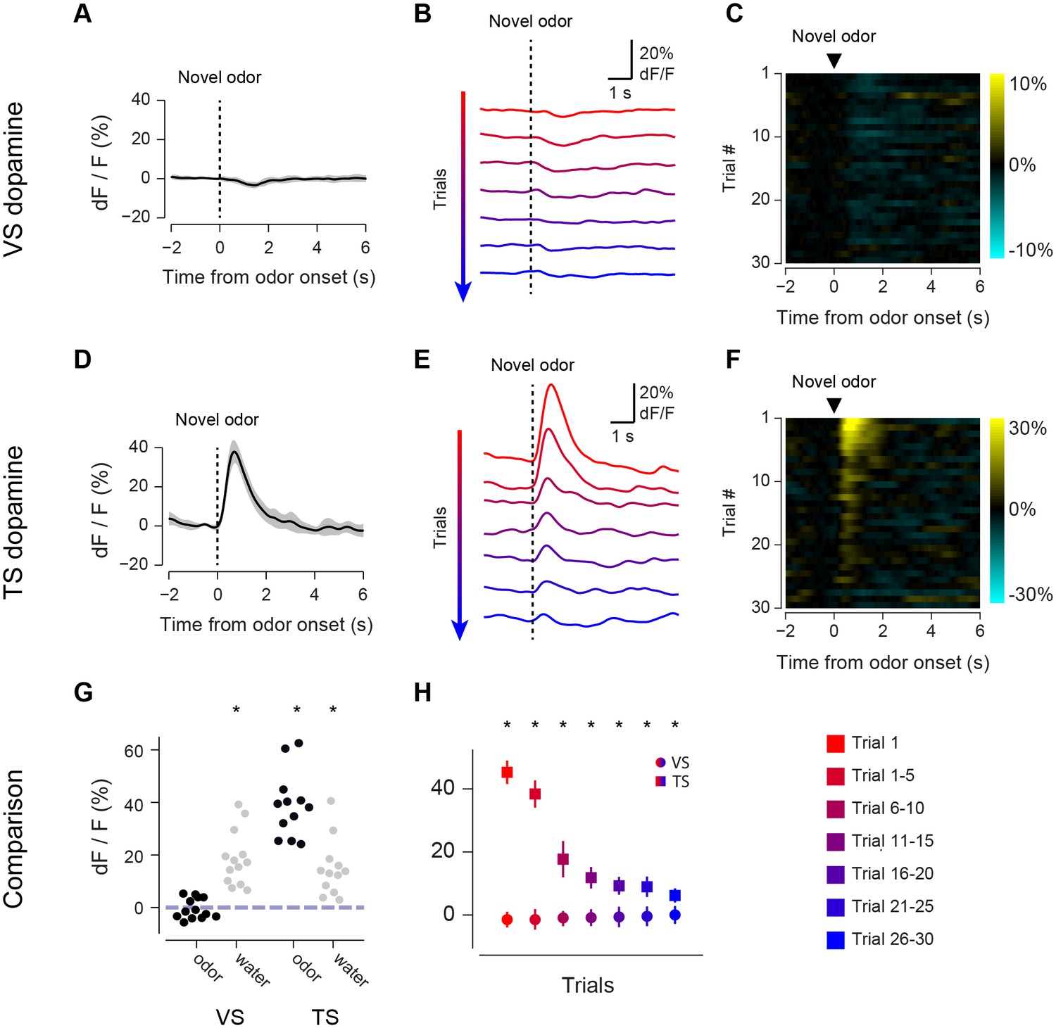
Responses to novel odors in VS and TS dopamine.
Comparison of VS and TS responses to novel odors in naïve animals. (A) Average response to the first presentation of a novel odor in VS dopamine, with SE bars. (B) Average responses over the course of the first 30 trials are shown in bins of 5 trials. (C) A heat map of responses to a novel odor over the course of a single session (each row is one trial) with yellow indicating an increase in signal and cyan indicating a decrease in signal. (D–F) TS dopamine responses to novel odors, plotted as in A–C. (G) Comparison of first-trial water responses in VS and TS (left) and first-trial responses to novel odors (right). See Materials and methods. (H) Time course of responses to a novel odor in VS (circles) and TS (squares) over the course of 30 trials in bins of 5 trials. This data was analyzed based on odor decay rates to show that there was no large effect of odor decay in Figure 2—figure supplement 1. Motion artifacts were examined in Figure 2—figure supplement 3. GCaMP signal decay was measured in Figure 2—figure supplement 2. Finally, response latencies are shown in Figure 2—figure supplement 4.
Figure 2—figure supplement 1
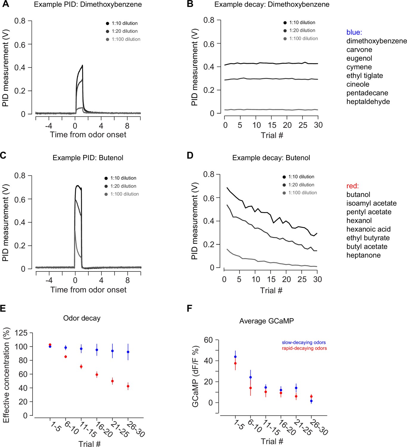
PID measurements of odor decay rates.
(A–B) An example of PID measurements from an odor with a slow rate of decay: dimethoxybenzene. Plot on the left is a single trial PID measurement after 1:10 dilution, 1:20 dilution, or 1:100 dilutions. Plot on the right is the decay of the PID measurement over a session. (C–D) An example of PID measurements from an odor with a fast rate of decay: butenol. Plots are the same as above. (E) The average decay rate of slow decaying odors (blue) and fast decaying odors (red) over a session. (F) Average TS dopamine signal in response to novel odors with a slow decay rate (blue) or fast decay rate (red). Data from 2 hr is plotted, separated based on odorant.
Figure 2—figure supplement 2

GCaMP response decay within sessions.
The average GCaMP responses to free water in VS (A, D, G), free water in TS (B, E, H), and familiar odors in TS (C, F, I) are plotted. Top row: average traces over the course of a session (~45 min) with early responses plotted in blue and late responses plotted in red. Middle row: average peak responses plotted over the course of a session, with a linear fit of the data plotted in grey. Bottom row: heat maps of the average responses, with yellow indicating an increase in signal and cyan indicating a decrease in signal.
Figure 2—figure supplement 3
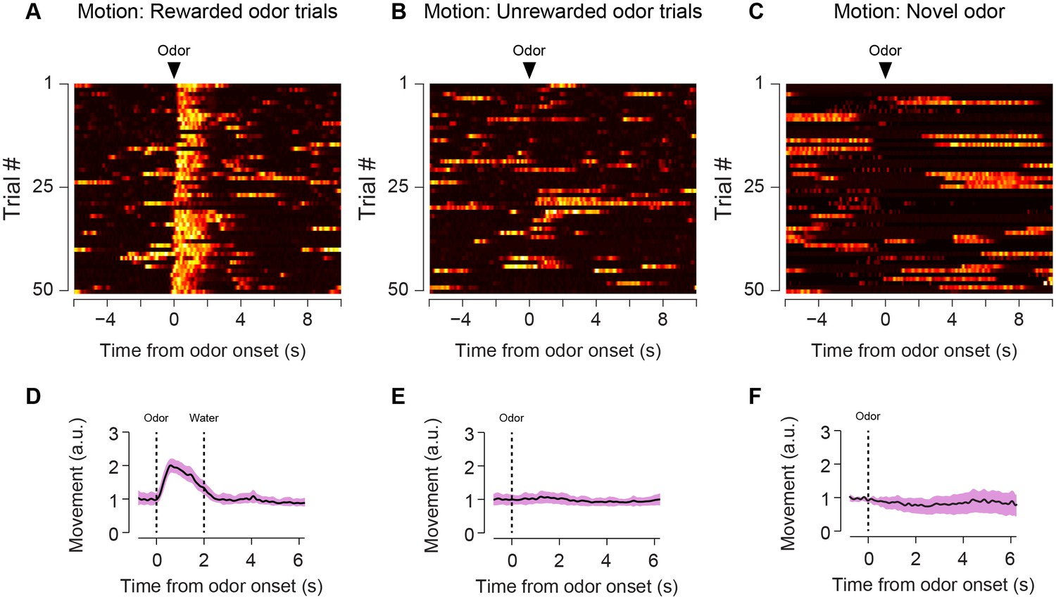
Animal body movement during trials.
Heat maps from example sessions showing the total body movement following familiar odors predicting reward (A), familiar odors predicting nothing (B), and novel odors predicting reward (C). The average trace from six animals is shown for each of these trial types (D–F) along with standard error.
Figure 2—figure supplement 4

Latency of GCaMP responses to novel odors in TS.
The first 5 TS dopamine GCaMP responses to a novel odor were compared across 12 naïve animals. (A) A histogram of the response latencies from each of the trials. The median response latency is 140 ms (see Materials and methods). The bold line represents the cumulative probability that a response was observed at that time, in any trial. (B) An example trace from a single trial (green) as well as the average trace among all trials (five trials per animal used, 12 animals total).
Figure 3 with 1 supplement
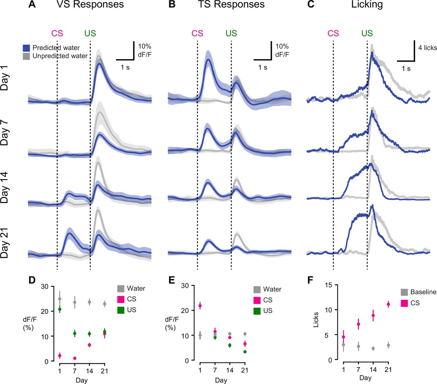
Opposite dynamics of VS and TS dopamine during initial learning of new odor-reward associations.
Learning dynamics for VS dopamine (A) and TS dopamine (B) over the course of 3 weeks of training, as naïve animals learn an association between an odor and reward. Odor onset (CS) and water delivery time (US) are shown as dotted lines. Responses are compared on day 1, day 7, day 14, and day 21. The average traces are plotted in blue (predicted reward) and black (unpredicted reward), with the standard error of the mean (SEM). Individual animals’ responses can be found in Figure 3—figure supplement 1. (C) Average licking in response to reward-predicting odor (blue) compared to average licking in response to unexpected reward (black). (D) A quantification of the CS and US responses in VS from the above traces, over training compared to responses to unexpected water (black). (E) A quantification of the CS and US responses in TS from the above traces, over training, compared to responses to unexpected water (black). (F) The average number of anticipatory licks in the period between odor presentation and water delivery, compared over days of training.
Figure 3—figure supplement 1
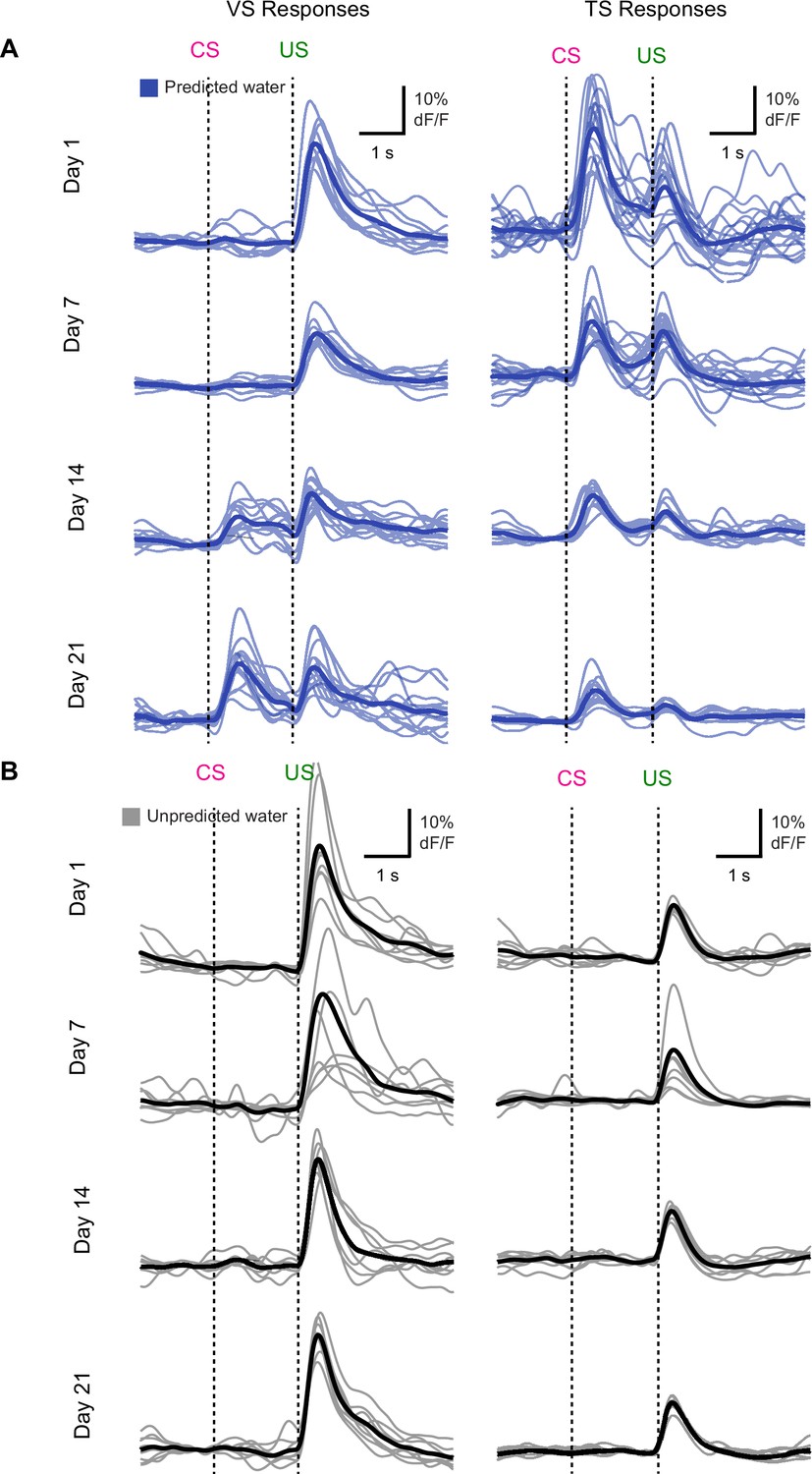
Individual traces during initial learning of new odor-reward associations.
Individual animals’ responses to (A) predicted water (blue) and (B) unpredicted water (black) over the course of learning. Average among animals is shown as a slightly darker trace. Each individual trace represents the average among trials for a single session, for that animal. The session day is indicated on the left.
Figure 4 with 3 supplements
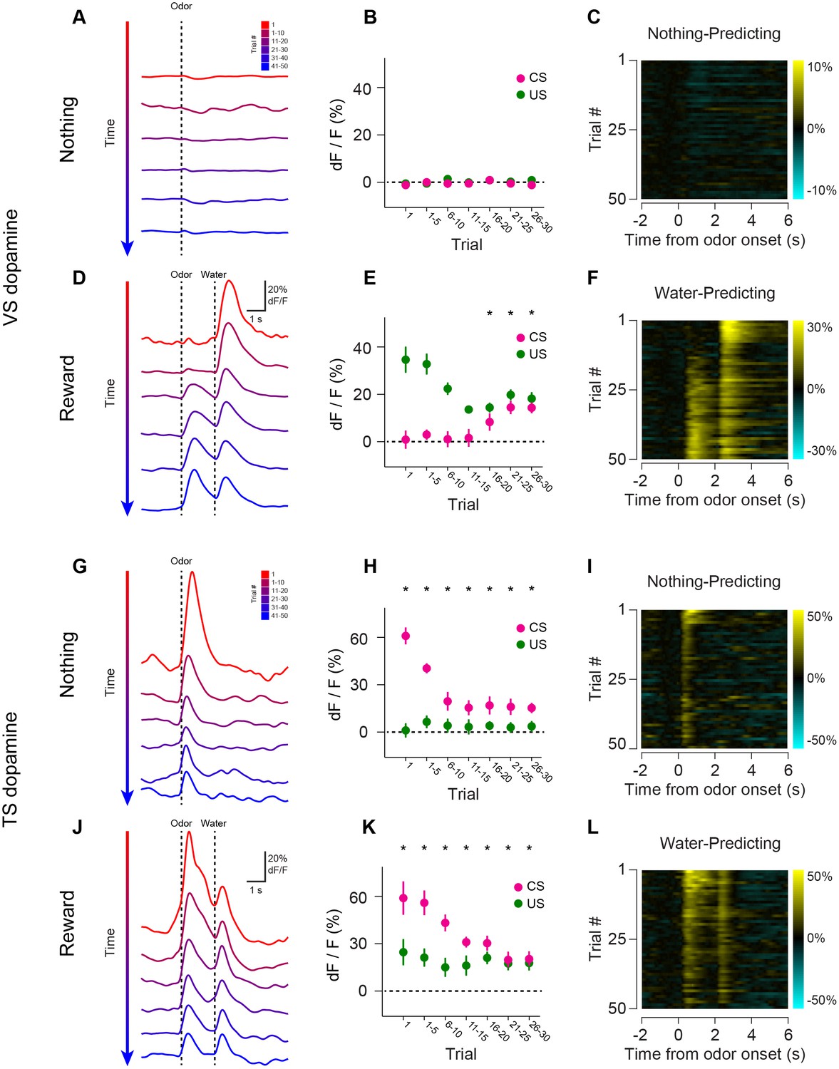
Opposite dynamics of VS and TS dopamine during repeated learning of new odor-reward associations.
Responses to new cues predicting nothing (A–C) or water (D–F) in VS. Responses to new cues predicting nothing (G–I) or water (J–L) in TS. Responses to aversive air puffs are found in Figure 4—figure supplement 1 and quantified in Figure 4—figure supplement 2. In the panels on the left, trials are color-coded such that red indicates the first trial and blue indicates the last trials of the session. Trials were quantified in bins of 5 trials. The middle panels show the average CS (magenta) and US (green) responses over the course of a session, again quantified in bins of 5 trials. The panels on the right are heat maps, where every line is a single trial. In these heat maps, yellow indicates an increase in signal and cyan indicates a decrease. Odor discrimination latency is quantified in Figure 4—figure supplement 3.
Figure 4—figure supplement 1
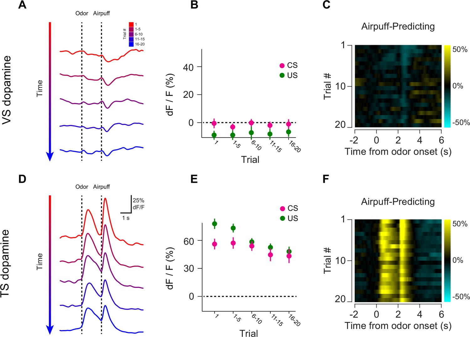
Opposite dynamics of VS and TS dopamine during repeated learning of new odor-puff associations.
Responses to new cues predicting air puff in VS (A–C). Responses to new cues predicting air puff in TS (D–F). In the panels on the left, trials are color-coded such that red indicates the first trial and blue indicates the last trials of the session. Trials were quantified in bins of 5 trials. The middle panels show the average CS (magenta) and US (green) responses over the course of a session, again quantified in bins of 5 trials. The panels on the right are heat maps, where every line is a single trial. In these heat maps, yellow indicates an increase in signal and cyan indicates a decrease.
Figure 4—figure supplement 2
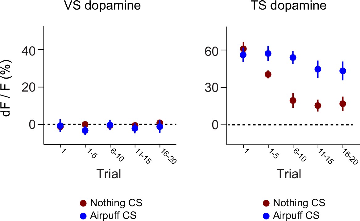
Dynamics of responses to puff-predicting odors.
A comparison of the CS responses to novel air puff predicting odors and novel odors predicting nothing in VS dopamine (left) and TS dopamine (right).
Figure 4—figure supplement 3
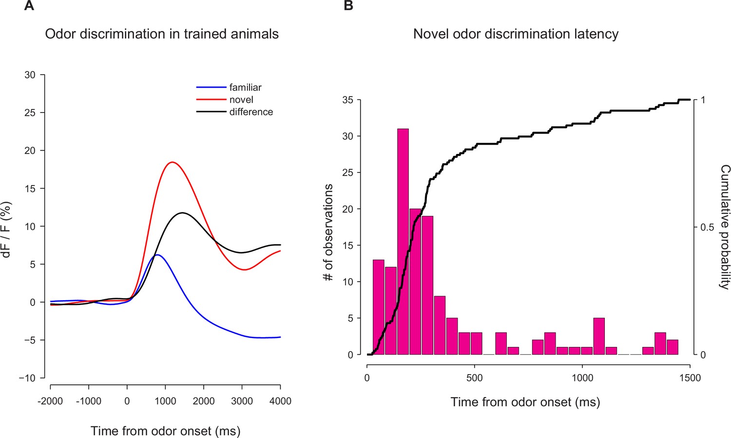
Novel odor discrimination latency in TS dopamine.
A quantification of the latency of discrimination between novel and familiar odors in the TS dopamine responses recorded from trained mice. (A) The average TS dopamine responses to novel (red) or familiar (blue) odors. The black trace is the difference between the familiar and novel odors – indicating the time course of discrimination. (B) A histogram of the latencies of discrimination. The median latency is 170 ms. The bold line represents the cumulative probability that discrimination had occurred by that time.
Figure 5 with 2 supplements
Dynamics of anticipatory licking behaviors and VS and TS dopamine.
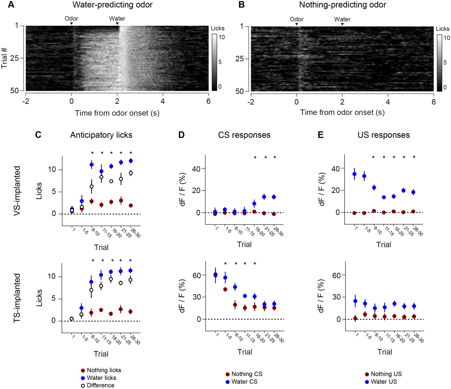
Licking in response to new odors predicting reward (A) or no outcome (B) over the course of a session, in animals that have been trained with many new odor associations, as in Figure 4 (see Materials and methods). Separate plots for VS-implanted mice and TS-implanted mice are shown in Figure 5—figure supplement 1. (C) A quantification of the number of anticipatory licks elicited by each odor in VS-implanted animals (left) and TS-implanted animals (right). The difference between licks following a rewarding odor and an unrewarding odor are shown as open circles. (D) A comparison of the CS responses to rewarding and unrewarding new odors in VS dopamine (left) and TS dopamine (right). (E) A comparison of the US responses to either predicted water or predicted nothing in VS dopamine (left) and TS dopamine (right). The relationship between GCaMP responses in VS and TS and anticipatory licking is shown in Figure 5—figure supplement 2.
Figure 5—figure supplement 1
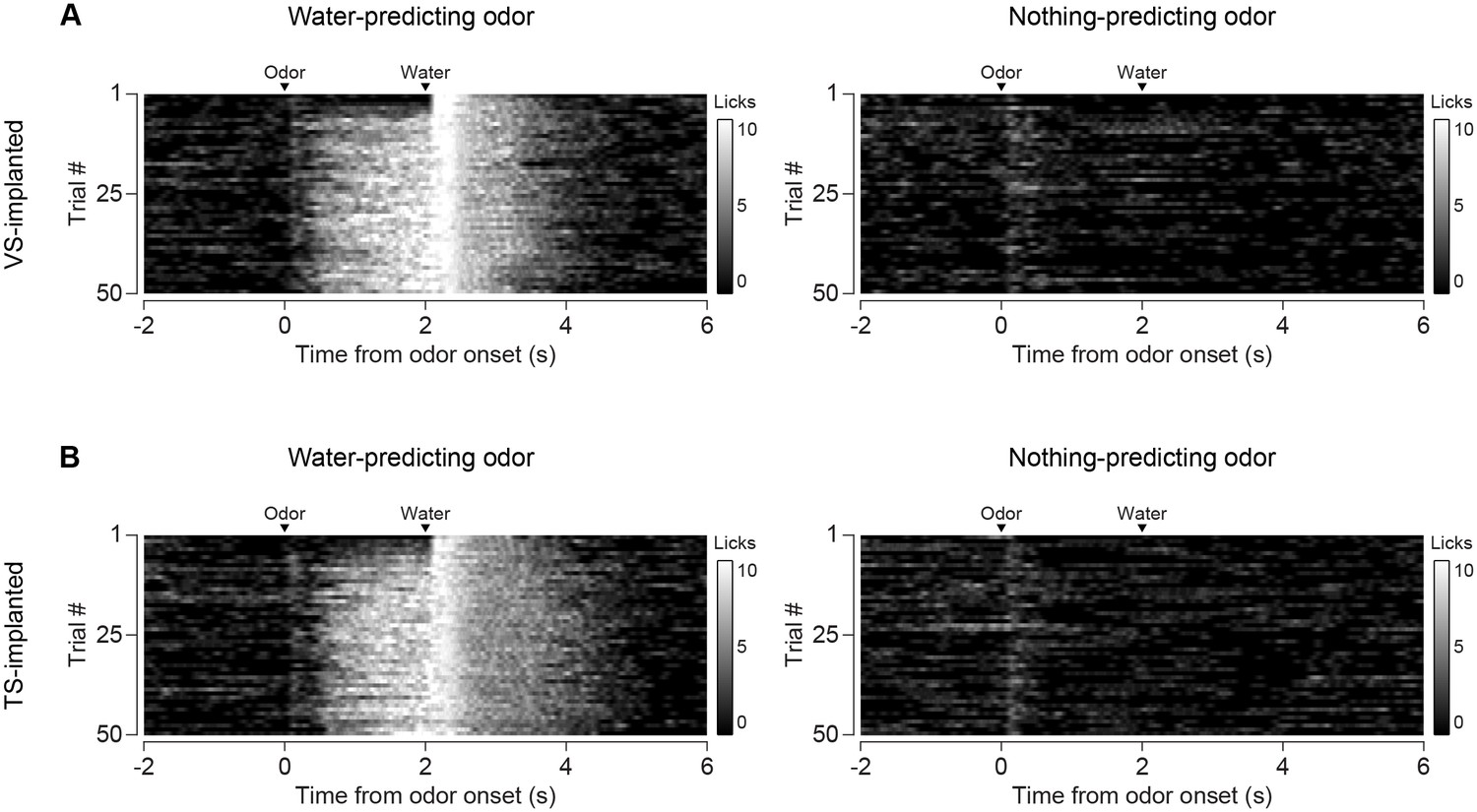
Comparison of licking in VS-implanted and TS-implanted animals.
(A) Licking in response to new odors predicting reward (left) or no outcome (right) in animals with an optical fiber implanted in VS. (B) Licking in response to new odors predicting reward (left) or no outcome (right) in animals with an optical fiber implanted in TS.
Figure 5—figure supplement 2
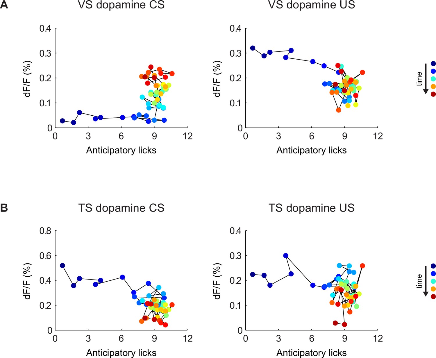
Relationship between CS/US responses and anticipatory licking.
The relationship between VS dopamine signals (A) or TS dopamine signals (B) and anticipatory licking. The left panels are plots of CS (cue) responses and anticipatory licking. The panels on the right are plots of US (water) responses and anticipatory licking. Markers are colored based on the order of the trials, from blue (first trial) to red (last trial). Trials are connected with thin black lines based on the order in the session.
Figure 6 with 2 supplements
Responses to rewarding, aversive and neutral stimuli in VS and TS dopamine.
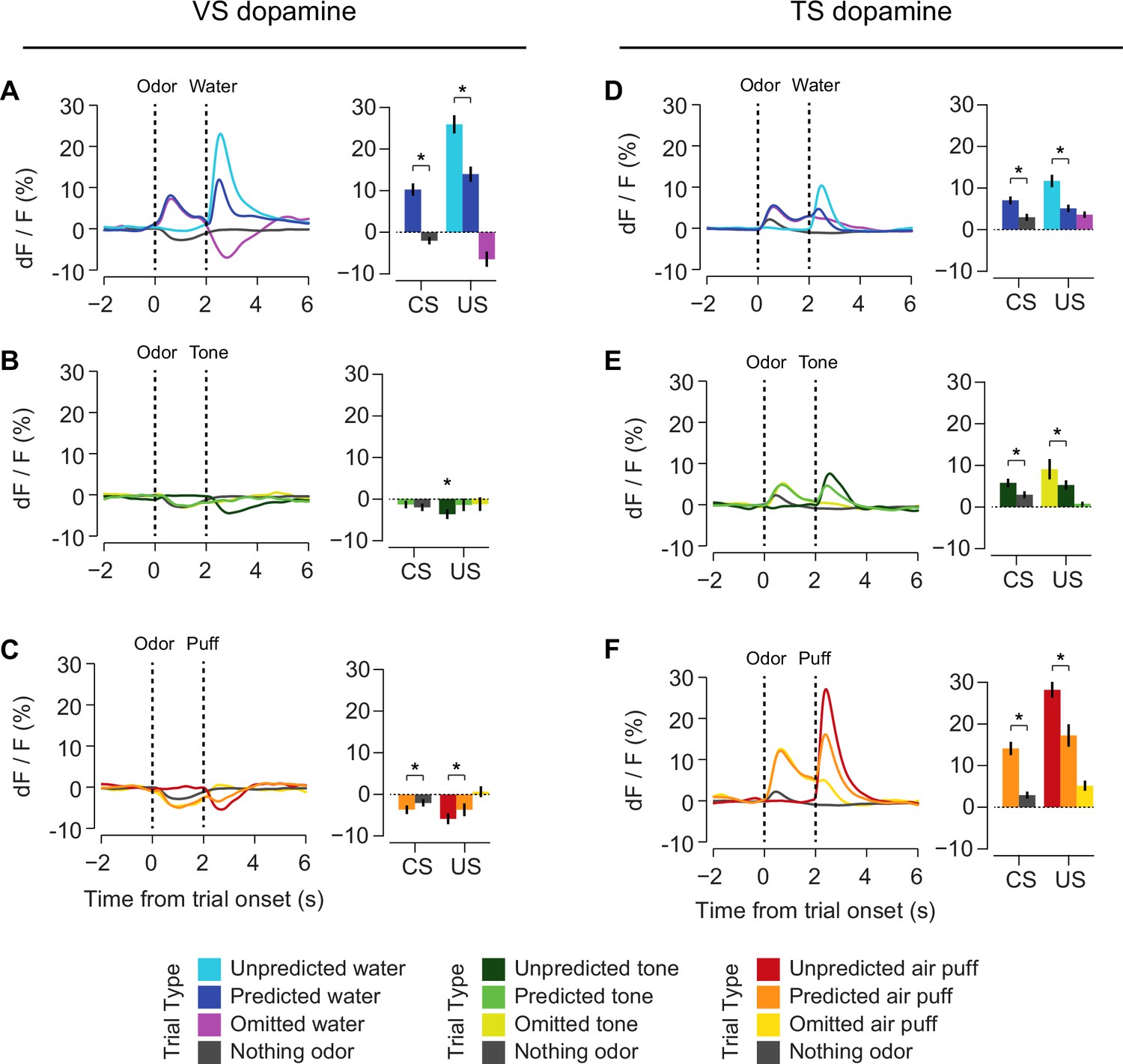
Dopamine responses to water (A), tone (B), and air puff (C) in the ventral striatum and the posterior tail of the striatum (D–F). Plots of average traces from each region contain dotted lines indicating odor (CS) and outcome (US) delivery times. (A, D) Responses to unpredicted reward (cyan), predicted reward (blue), omitted reward (purple), and nothing odor (grey) are plotted in the left panels. For each trace, a quantification of the average peak response to the CS / US is shown on the right. (B, E) Responses to unpredicted tone (dark green), predicted tone (light green), omitted tone (yellow), and nothing odor (grey) are plotted in the left panels. For each trace, a quantification of the average peak response to the CS / US is shown on the right. (C, F) Responses to unpredicted air puff (red), predicted air puff (orange), omitted air puff (yellow), and nothing odor (grey) are plotted in the left panels. For each trace, a quantification of the average peak response to the CS / US is shown on the right. Data from individual sessions is shown in Figure 6—figure supplement 2. Behavioral responses to the tone are shown in Figure 6—figure supplement 1.
Figure 6—figure supplement 1
Behavioral quantification of tone responses.
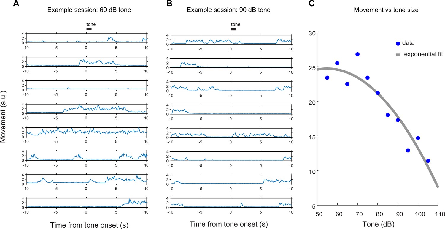
Total body movement in response to tones of different volumes. The tone used in Figure 6 was 55 dB, for comparison. (A) An example of single-trial responses to a quiet (60 dB) tone. (B) An example of single-trial responses to a relatively loud (90 dB) tone. (C) A plot of the average total body movement in response to tones of different volumes, with a lower number indicating a higher instance of freezing or remaining still.
Figure 6—figure supplement 2

Individual session data.
A heat map of the average responses from each session (from all animals) to odors predicting reward (left) or no outcome (right). The top panels are responses in VS and the bottom panels are responses in TS. Each row is the average for a session.
Figure 7 with 2 supplements

Maps of dopamine responses in VS and TS.
The distribution of responses to novelty (A), reward (B), familiar odor predicting nothing (C), air puff (D), and reward omission (E). In the left panels, a 3D view of the average response from each animal. Novelty responses are the first responses to a novel odor either in the naïve case (i.e. Figure 2) or the trained case (i.e. Figure 4). Reward responses are the average response to unpredicted reward. Nothing responses are the response to cues predicting no outcome. Air puff responses are the average response to unpredicted air puff. Omission responses are the average response to the omission of expected water. In the middle panels, coronal max projections are shown from the 3D view. On the right, the correlation between signals from the fibers and their positions on the A-P axis is shown, along with a yellow line indicating the best fit. The plots of these responses are shown for VS, DMS, DLS, and TS in Figure 7—figure supplement 2. Examples of the whole-brain images used to find recording sites are shown in Figure 7—figure supplement 1.
Figure 7—figure supplement 1
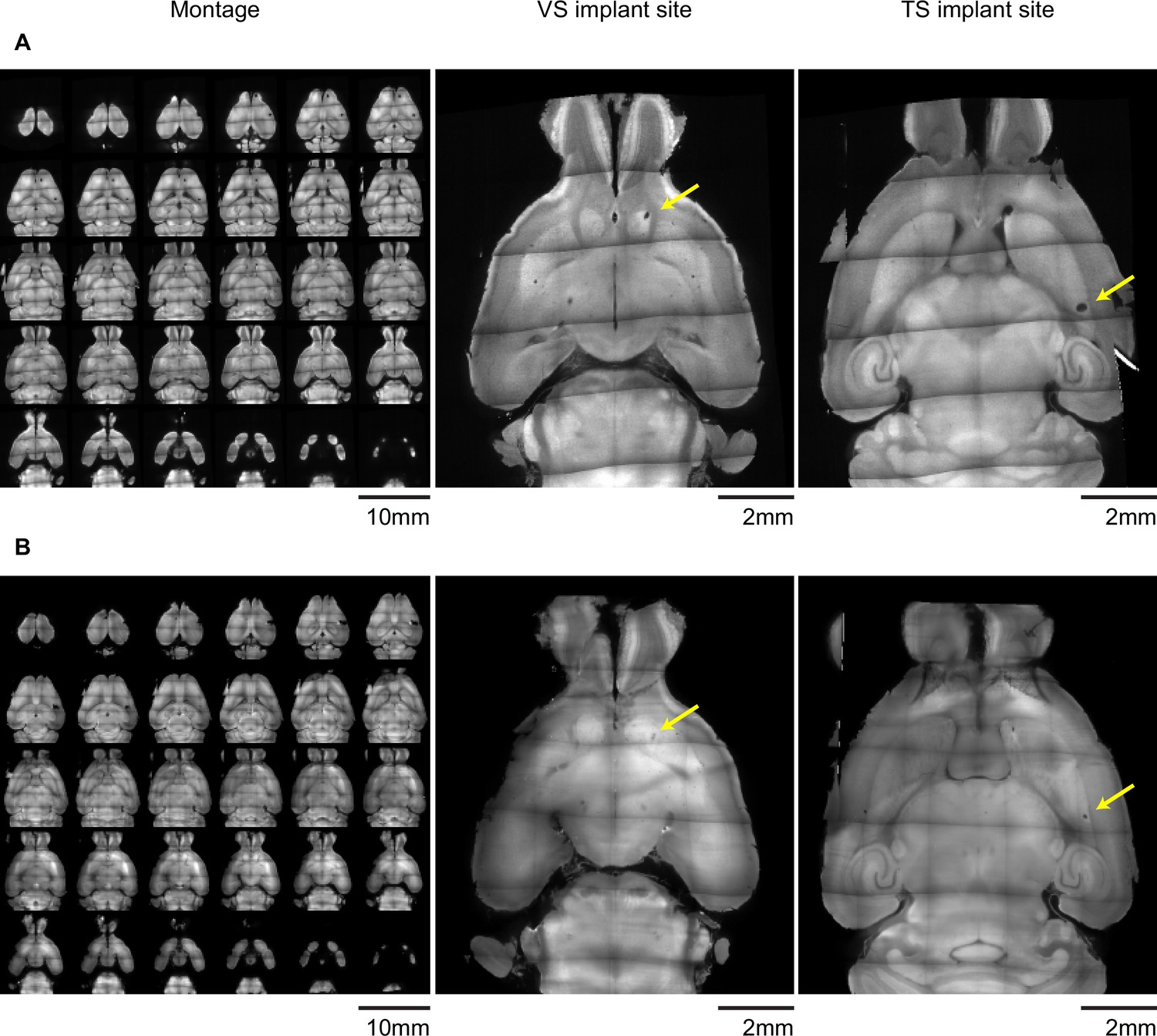
Examples of light-sheet images of cleared brains used to determine fiber locations.
Example autofluorescence images used to find the position of (A) 400 µm diameter or (B) 200 µm diameter optic fiber implants after clearing with CLARITY and imaging with a light sheet microscope. Panels on the left are horizontal optical slices, and the panels on the left are enlarged views of slices near the tip of each implanted fiber. Yellow arrows denote the position of the implant. Both example brains have implants in both VS and TS.
Figure 7—figure supplement 2
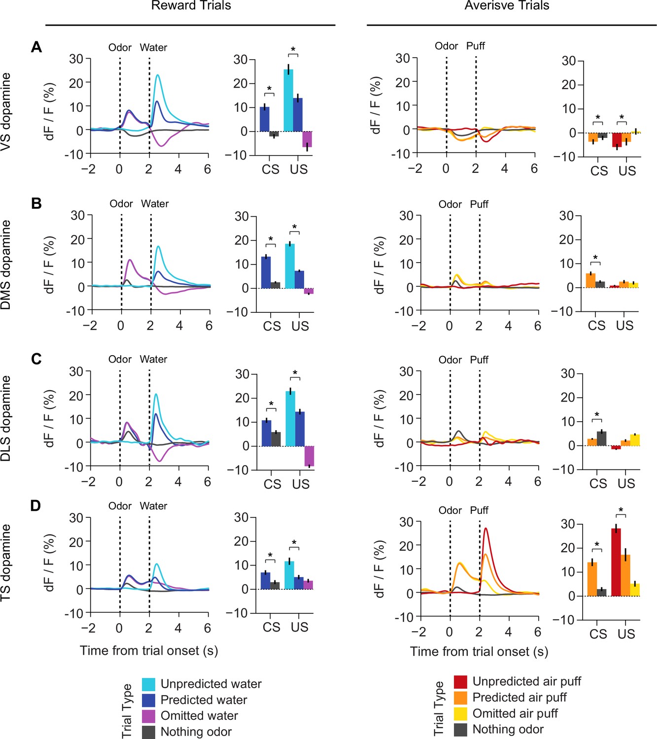
Responses to rewarding and aversive stimuli in VS, DMS, DLS, and TS.
A comparison of responses to water, water predicting cues, and water omission (left panels) with responses to air puff, airpuff predicting cues, and airpuff omission (right panels), in (A) VS dopamine, (B) DMS dopamine, (C) DLS dopamine, and (D) TS dopamine. Averages among all sessions and all animals are plotted on the left in each panel, and a quantification of the peak responses to each stimulus / outcome are plotted on the right.
Download links
A two-part list of links to download the article, or parts of the article, in various formats.
Downloads (link to download the article as PDF)
Open citations (links to open the citations from this article in various online reference manager services)
Cite this article (links to download the citations from this article in formats compatible with various reference manager tools)
Opposite initialization to novel cues in dopamine signaling in ventral and posterior striatum in mice
eLife 6:e21886.
https://doi.org/10.7554/eLife.21886


