Sensitivity to image recurrence across eye-movement-like image transitions through local serial inhibition in the retina
- University Medical Center Göttingen, Bernstein Center for Computational Neuroscience Göttingen, Germany
- Max Planck Institute of Neurobiology, Germany
Figures
Figure 1
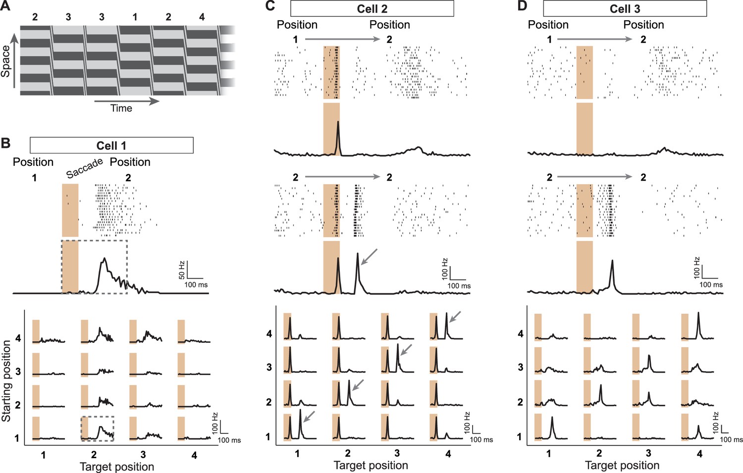
Sensitivity to image recurrence by retinal ganglion cells under saccade-like image shifts.
(A) Space-time representation of the saccade stimulus. The stimulus consisted of a spatial grating that was repeatedly shifted in a saccade-like fashion during 100 ms and then stopped randomly at one out of four different grating positions, where it then remained fixed for 800 ms before the next shift. The sequence of fixated grating positions, which are numbered from 1 to 4, is indicated in the top row. (B) Top: Raster plot and firing rate profile, obtained as the peristimulus time histogram (PSTH), for a ganglion cell (Cell 1) under shifts from grating position 1 to position 2. The saccade-like transition period is marked by the shaded region. Bottom: Firing rate profiles of the same cell for all 16 transitions between the four grating positions. Data are displayed for 400 ms, following transition onset. For comparison, the considered time window is shown by a dashed rectangle in the PSTH above. The fixation positions before and after the saccade-like transition are denoted as ‘starting position’ and ‘target position’, respectively. (C) Response patterns of a sample cell (Cell 2) with sensitivity to image recurrence (IRS cell). Raster plots and PSTHs are shown for transitions to grating position 2, starting either from position 1 (top) or from position 2 (center). Bottom: Firing rate profiles of this cell for all 16 transitions. The IRS response is apparent by the post-transition firing rate peak for traces along the diagonal of this matrix (marked by small arrows). (D) Same as (C) for another sample cell (Cell 3) with sensitivity to image recurrence, but without a response during the transition itself.
Figure 2
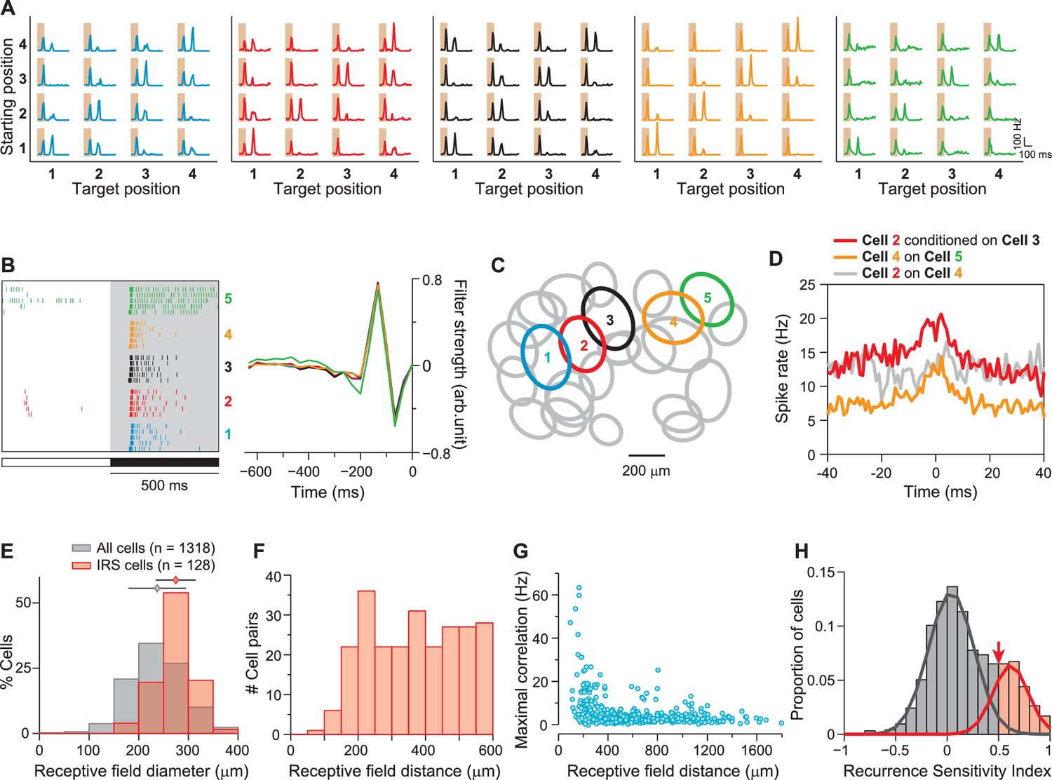
IRS cells show homogeneity in general response characteristics.
(A) Responses of five simultaneously recorded sample IRS cells to the 16 saccade-like transitions. (B) Raster plots for repeated steps in light intensity (left) and temporal filters obtained as spike-triggered averages under full-field white-noise stimulation (right) for the five sample IRS cells. (C) Receptive field outlines of the five sample IRS cells (colored ellipses), together with all other receptive fields obtained in the same recording (gray ellipses). (D) Spike-timing correlations of spikes in pairs of IRS cells from among the five sample cells. (E) Distribution of receptive field sizes of IRS cells (red) from all recordings, compared to the distribution for all recorded cells (gray; 48 recordings). (F) Receptive field center distances of pairs of IRS cells. (G) Spike-time correlations of 456 pairs of IRS cells plotted against the receptive field center distance. (H) Recurrence Sensitivity Index () of 963 cells from 48 recordings included for analysis (see ‘Materials and methods’ for details). Cells with were considered as IRS cells (red bars). The lines show a fit by a two-component Gaussian mixture model.
Figure 3 with 1 supplement
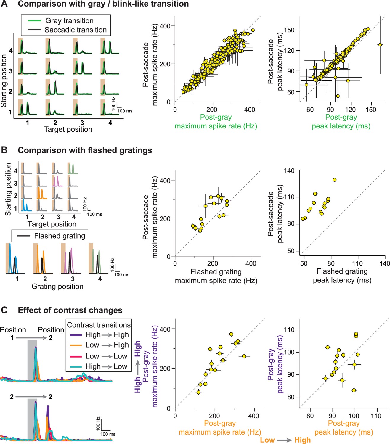
Stimulus history dependence of IRS responses.
(A) Comparison of responses from a sample IRS cell (left) for saccade-like transitions (black traces) and transitions masked by a gray screen of mean illumination (green traces) as well as population analysis of the maximum firing rate and its latency for the two transition types (right). For the population analysis, each data point represents the average for a single cell over the four grating positions with equal starting and target position, and error bars denote standard errors, but are smaller than the symbol size for many data points (N = 209 cells from 48 recordings). (B) Comparison of responses from a sample IRS cell (left) for saccade-like transitions of a recurrent grating (colored traces) and for flashing the same grating in isolation (black traces) as well as population analysis as in (A) of the maximum firing rate and its latency (right; N = 15 cells from five recordings). The flashed gratings were preceded by mean-intensity illumination, and their responses were aligned to the onset of the new fixation in the saccade-like transitions. (C) Responses of a sample IRS cell (left) for transitions that included random changes in contrast between a high (60%) and low (30%) level as well as population analysis of the maximum firing rate and its latency as in (A) for the transitions to the high-contrast target images (right; N = 15 cells from five recordings).
Figure 3—figure supplement 1
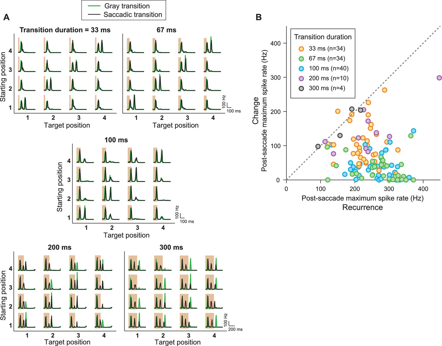
IRS responses are robust to variations of transition duration.
(A) Firing rate profiles for a sample IRS cell in response to the saccade stimulus with different durations of the transition period, ranging from 33 ms to 300 ms, for saccadic (black traces) and masked (green) transition. The variations in transition duration were accompanied by corresponding differences in the speed of the saccade-like shifts. The characteristic IRS responses are visible in all cases. Note, though, that longer saccade-like shifts produced additional intermediate activity peaks. Apparently, the sequence of bright and dark illumination is now slow enough so that the neurons can follow and produce transient activation, for example, when the grating position temporarily matches the starting position during the saccadic transition. For example, for 300 ms shifts, the transition from position 1 to 3 yields two response peaks in addition to the transition-onset peak, in agreement with the fact that the transition here goes through 2.5 grating periods. For the transition from position 3 to 1, the grating only goes through 1.5 periods, and there is correspondingly only one additional peak. Furthermore, this explanation is in agreement with the fact that the masked transitions do not lead to intermediate activity peaks. (B) Population analysis of the post-saccade firing rate peaks under ‘Recurrence’ (equal starting and target position) and ‘Change’ (different starting and target position). Data come from a total of n = 40 cells from five recordings, for which typically a subset of transition durations was tested.
Figure 4 with 1 supplement
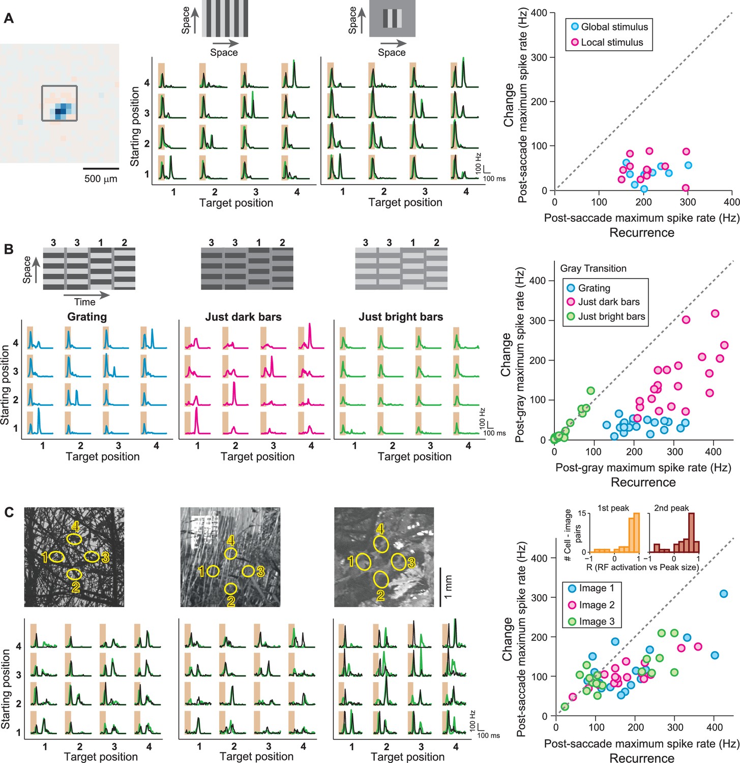
IRS responses are robust to spatial stimulus structure.
(A) Influence of spatial extent of the stimulus. Left: Receptive field of a sample IRS cell. The outlined square shows the region of a local saccade stimulus. Middle: Firing rate profile of the sample IRS cell for the standard saccade stimulus, displayed over the entire screen, and for a smaller stimulation area of 480 µm x 480 µm. Responses under masked transitions by a gray screen are shown in green. Right: Population analysis (N = 12 cells from three recordings). For each recorded IRS cell, the maximum firing rate after onset of the target image was averaged over transitions with equal starting and target position (‘Recurrence’, x axis) and for the other transitions, where starting and target position differed (‘Change’, y axis). (B) Differential effects of bright and dark grating components. Left: Responses from a sample IRS cell to the standard grating stimulus and to gratings that contained only the dark or bright bars, all for transitions with a gray screen. The space-time representations of the stimuli are shown on top. Right: Population analysis (N = 21 cells from five recordings) as shown in (A). (C) Responses of three IRS cells (bottom, black traces) to saccade-like shifts of natural images (top). Ellipses in the images denote the receptive field outlines at the four fixation positions. Transitions lasted 100 ms and either occurred linearly between two fixation positions (starting position different from target position) or were composed of a shift to the center during the first 50 ms, immediately followed by a shift back to the starting position (equal starting and target position). For comparison, responses where the image was blurred during the transition are shown in green. Right: Population analysis of IRS cell responses to three natural images (N = 17 cells from four recordings). Inset: Distributions of correlation coefficients between the size of the first firing-rate peak and the integrated darkening in the receptive field at transition onset (left) as well as between the size of the second firing-rate peak and the integrated darkening in the receptive field at fixation onset (right).
Figure 4—figure supplement 1
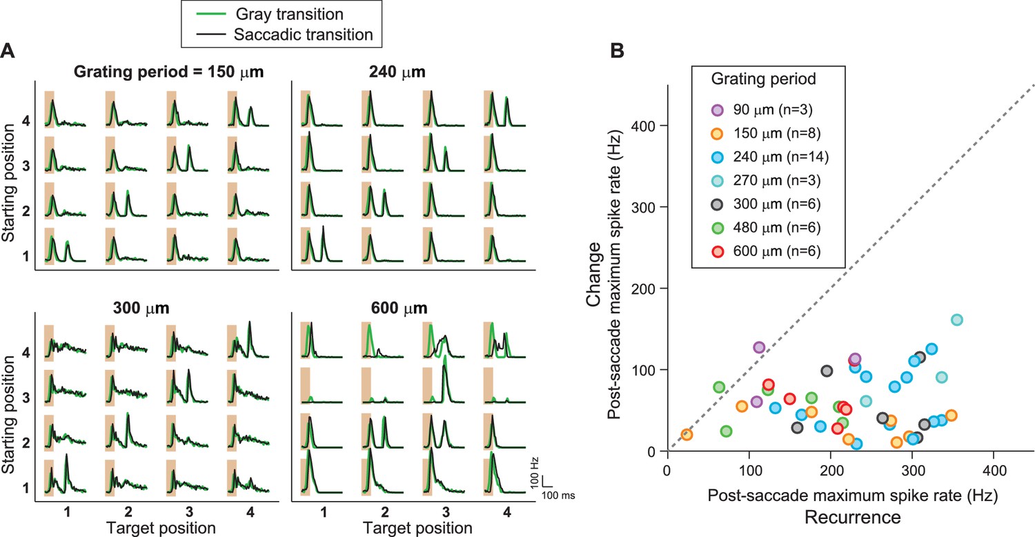
IRS responses are robust to variations of spatial stimulus scale.
(A) Firing rate profiles for a sample IRS cell in response to the saccade stimulus at different spatial periods of the grating, ranging from 150 µm to 600 µm. The characteristic response for equal starting and target position is visible in all cases; only for gratings with bars wider than the receptive field center (cf. spatial period of 600 µm) did the responses reveal dependences on the specific grating positions prior to or after the transition. (B) Population analysis of the post-saccade firing rate peaks under ‘Recurrence’ (equal starting and target position) and ‘Change’ (different starting and target position). Data come from a total of n = 17 cells from six recordings, for which typically a subset of grating periods was tested.
Figure 5
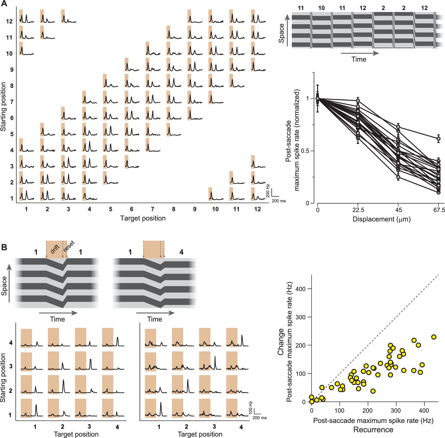
IRS responses are sensitive to small net translations and microsaccade-like image resets.
(A) Left: Responses of a sample IRS cell to a stimulus with fine net displacements between starting and target position, corresponding to a resolution of 30° of grating phase or 22.5 µm translation on the retina. Top right: Space-time representation of the stimulus. Bottom right: Population analysis of the dependence of the averaged post-transition maximum firing rate on the net displacement between starting and target image (N = 22 cells from seven recordings). Firing rates were normalized to the value obtained for zero net displacement, and error bars correspond to standard errors. Lines connect data points of individual IRS cells. (B) Left: Responses of two IRS cells (bottom) to drift-reset stimulus motion, as schematically depicted on top, which can represent a correct reset (left) or a reset that is too short (right) or too far. Right: Population analysis of responses to the drift-reset stimulus (N = 50 cells from five recordings).
Figure 6
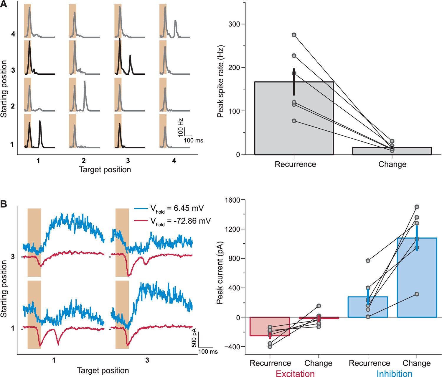
Synaptic inputs that mediate IRS responses.
(A) Left: Responses of a sample IRS cell recorded in loose-patch mode. Right: Population analysis of the post-transition firing rate peaks of IRS cells recorded in loose-patch mode (N = 6 cells). (B) Left: Currents of the same sample cell as in (A), recorded in whole-cell mode. Note that here the stimulus is restricted to transitions between two fixation positions, corresponding to the data displayed in bold in (A). Note further that the sequence of fixation positions was not randomized in these experiments, but followed a fixed, alternating sequence of change and recurrence of grating position. This explains the slight differences in the level of inhibitory currents before the transition. Right: Population analysis of excitatory and inhibitory current responses. The excitatory peak current was determined as the minimal current in the window from 100 to 250 ms after fixation onset under a holding potential near −70 mV and the inhibitory peak current as the maximal current at the same time point under a holding potential near 0 mV. Error bars in (A) and (B) show standard errors.
Figure 7
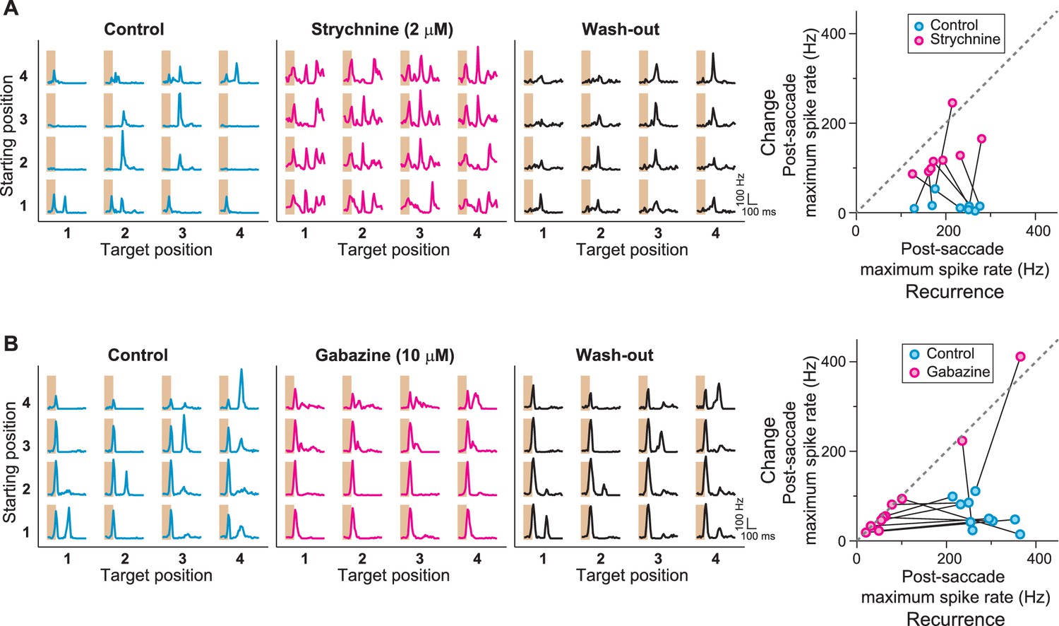
Role of GABAA- and glycine-mediated inhibition in generating IRS responses.
(A) Left: Firing rate profile of a sample IRS cell before, during, and after application of the glycine blocker strychnine. Right: Comparison of responses before (blue) and during drug application (magenta) for all recorded IRS cells. For each cell and condition, the maximum firing rate after onset of the target image was averaged over transitions with equal starting and target position (‘Recurrence’, x axis) and for transitions with different starting and target positions (‘Change’, y axis). Connected data points come from the same cell (N = 8 cells from three recordings). (B) Firing rate profiles of a sample IRS cell before, during, and after application of the GABAA blocker gabazine. Right: Comparison of responses before (blue) and during (magenta) drug application for all recorded IRS cells as in (A) (N = 10 cells from three recordings). The two cells with strong spike rate increases under gabazine for transitions of the ‘Change’ type displayed a strong broadening of the first response peak into the post-transition analysis window, but did not show distinct second response peaks.
Figure 8 with 2 supplements
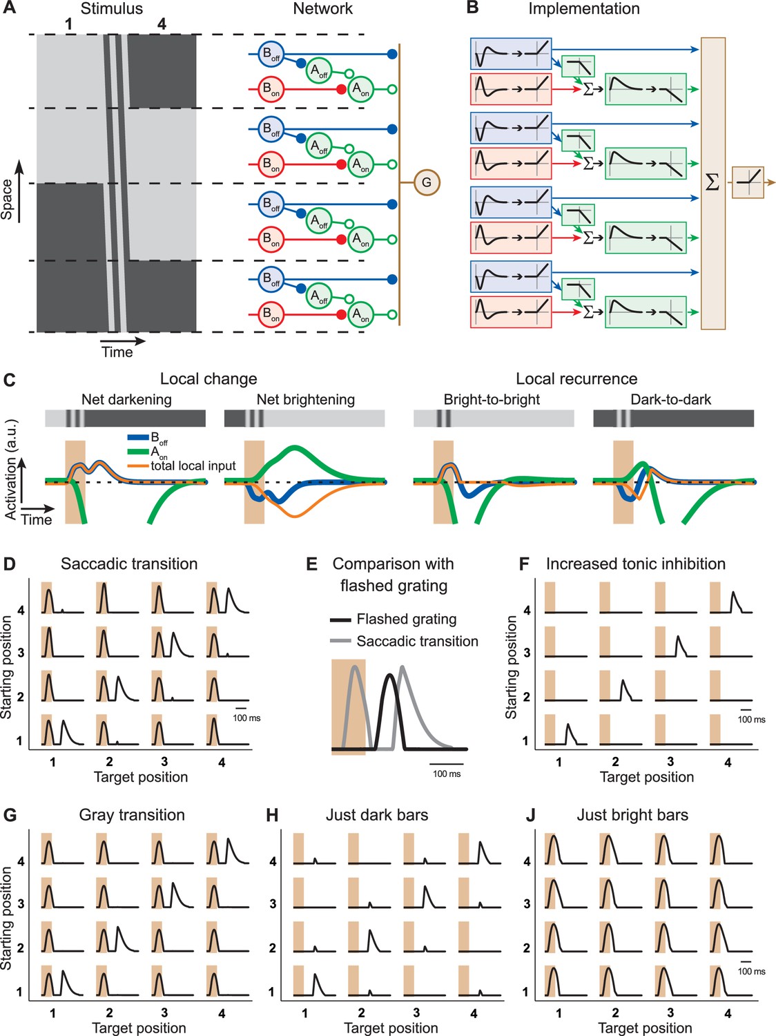
Computational model with local serial inhibition explains IRS responses.
(A) Schematic depiction of stimulus and model circuit. Left: Space-time representation of the stimulus for a sample transition from grating position 1 to 4. Right: Model circuit. The ganglion cell (G) receives excitatory input from Off-type bipolar cells (Boff) and inhibitory input from On-type amacrine cells (Aon), which are activated by On-type bipolar cells (Bon). In addition, these amacrine cells receive inhibition from Off-type amacrine cells (Aoff), which are activated by the Off-type bipolar cells. (B) Functional depiction of the model circuit. Bipolar cells are represented by temporal filters, shown here in the time domain, followed by a half-wave rectifying nonlinearity. Amacrine cells implement similar rectification, together with sign-inversion, and the Aon cell additionally applies a temporal low-pass filter and a non-zero threshold of rectification, accounting for tonic inhibition received by the ganglion cell. The ganglion cell is represented by a sum (Σ) of its inputs and another rectification stage. (C) Model responses of local interneurons. Activation curves of Off-type bipolar cells (blue) and On-type amacrine cells (green) are displayed for a saccade-like transition of the grating. The 100-ms transition is marked by the shaded areas. The corresponding local light intensity is indicated in the top row. Also shown is the resulting total input to the ganglion cell for each local stimulus (orange), which is obtained as the rectified Boff activity minus the rectified Aon activity. The activation curves of the On-type bipolar cells and Off-type amacrine cells are not displayed because they differ from those of the Off-type bipolar cells only by a sign inversion and a threshold, respectively. (D) Simulated firing rate profiles for the 16 saccade-like transitions. (E) Comparison of the model responses to a recurring grating and to the same grating flashed in isolation, analogous to the experimental data shown in Figure 3B. (F) Simulated firing rate profiles for the 16 saccade-like transitions with increased tonic inhibition supplied by the amacrine cell Aon, reproducing data where the spike burst during the transition itself was absent (cf. Figure 1D). (G) Simulated firing rate profiles for gray transitions (cf. Figure 3A). (H, J) Simulated firing rate profiles for stimuli with either only dark or bright bars (cf. Figure 4B).
Figure 8—figure supplement 1
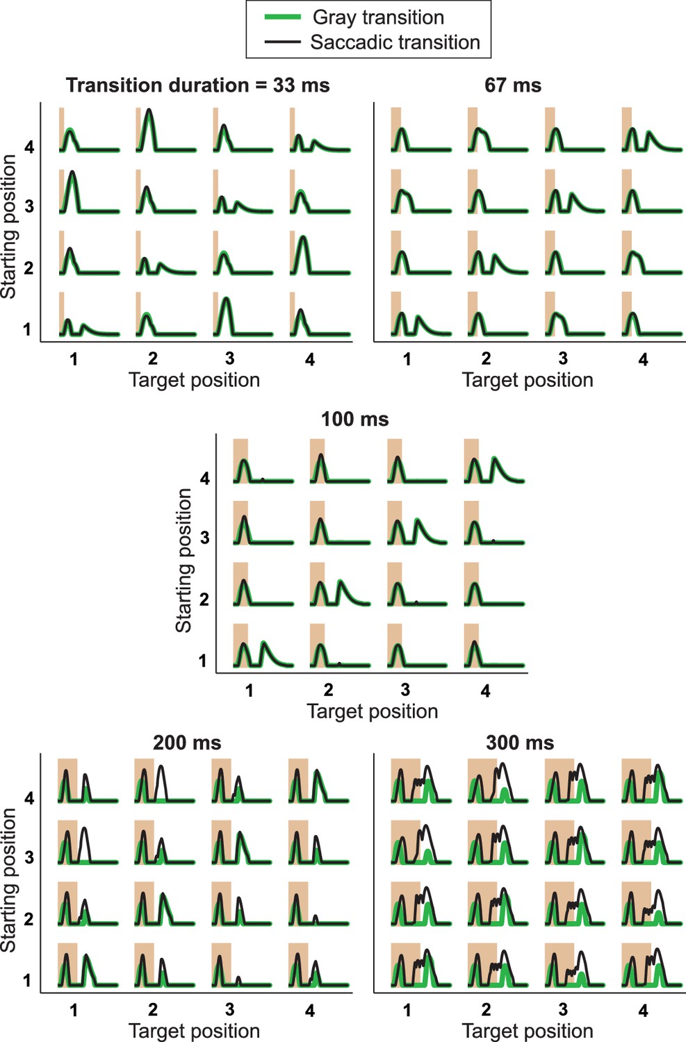
Responses from simulations of the IRS cell model under different transition durations.
The model of Figure 8 was applied to different transition durations from 33 ms to 300 ms, for both saccadic transitions (black traces) and transitions masked by background illumination (green), for comparison with experimental data (cf. Figure 3—figure supplement 1). Note that simulation results for 100-ms transitions are the same as in Figure 8D and G, although displayed with a different scale on the y axis, so that here all five plots can be shown with a fixed scaling and accommodate the larger response peaks for brief and long transitions. The responses to very brief and long transitions point to shortcomings of the model for processing rapid stimulus components. Apparently, the applied bipolar cell filters are too weakly activated under 33-ms transitions of recurring images. Furthermore, for longer transitions, the model is quite sensitive to the stimulus dynamics during a saccadic transition, producing a second response peak under 200-ms transitions for the transitions from positions 3 to 1 and 4 to 2, but not for the opposite transitions. Note that this asymmetry is connected to our implementation of the shift distance, which covers 1.5 grating cycles for the former transitions, but only 2.5 grating cycles for the latter. Masked transitions, on the other hand, which have no fast stimulus dynamics during the transitions, produce more robust IRS responses for longer transition durations, supporting the notion that the lack of appropriate dynamics for integrating rapid stimulus fluctuations causes the model’s deviations from data for short and long transitions.
Figure 8—figure supplement 2
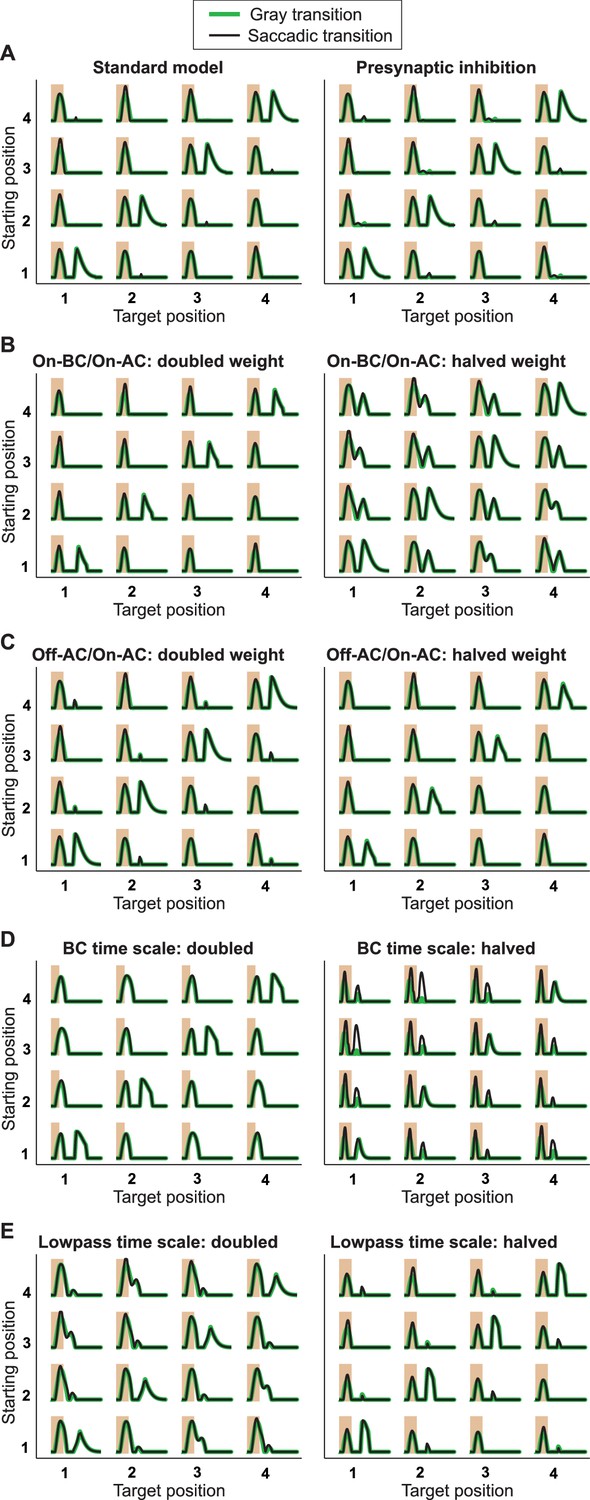
Responses from simulations of the IRS cell model under variations of parameters.
Robustness of the model of Figure 8 was tested by varying key parameters of the model and assessing the responses to the standard grating transitions, using both saccadic transitions (black traces) and transitions masked by background illumination (green). (A) The standard model (left) is compared to a model version (right) where the On-type inhibition acts presynaptically on the Off-type bipolar cells, that is, before rectification of the bipolar-cell input to the ganglion cell takes place. (B) Simulations with altered strength of the On-type inhibition, implemented by changing the weight for the connection from the On-type bipolar cell to the On-type amacrine cell. (C) Simulations with altered strength of the serial inhibition, implemented by changing the weight for the connection from the Off-type amacrine cell to the On-type amacrine cell. (D) Simulations with altered kinetics of stimulus filtering, obtained by simultaneously scaling all time-scale parameters of the bipolar cell stimulus filter. (E) Simulations with altered time scales of low-pass filtering in the On-type amacrine cell, implemented by simultaneously scaling all time-scale parameters of the low-pass filter.
Download links
A two-part list of links to download the article, or parts of the article, in various formats.
Downloads (link to download the article as PDF)
Open citations (links to open the citations from this article in various online reference manager services)
Cite this article (links to download the citations from this article in formats compatible with various reference manager tools)
Sensitivity to image recurrence across eye-movement-like image transitions through local serial inhibition in the retina
eLife 6:e22431.
https://doi.org/10.7554/eLife.22431


