Emergence of transformation-tolerant representations of visual objects in rat lateral extrastriate cortex
- International School for Advanced Studies (SISSA), Italy
- Istituto Italiano di Tecnologia, Italy
- Harvard Medical School, United States
Figures
Figure 1 with 2 supplements
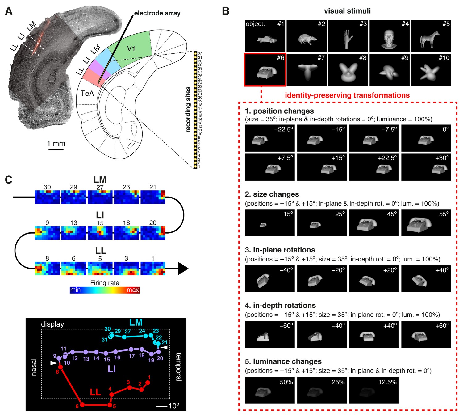
Experimental design.
(A) Oblique insertion of a single-shank silicon probe in a typical recording session targeting rat lateral extrastriate areas LM, LI and LL, located between V1 and temporal association cortex (TeA). The probe contained 32 recording sites, spanning 1550 µm, from tip (site 1) to base (site 32). The probe location was reconstructed postmortem (left), by superimposing a bright-field image of the Nissl-stained coronal section at the targeted bregma (light gray) with an image (dark gray) showing the staining with the fluorescent dye (red), used to coat the probe before insertion (see Figure 1—figure supplement 1). (B) The stimulus set, consisting of ten visual objects (top) and their transformations (bottom). (C) Firing intensity maps (top) displaying the RFs recorded along the probe shown in (A). The numbers identify the sites each unit was recorded from. Tracking the retinotopy of the RF centers (bottom: colored dots) and its reversals (white arrows) allowed identifying the area each unit was recorded from. Details about how the stimuli were presented and the RFs were mapped are provided in Figure 1—figure supplement 2. The number of neurons per area obtained in each recording session (i.e., from each rat) is reported in Figure 1—source data 1.
-
Figure 1—source data 1
Number of neurons per area obtained from each rat.
- https://doi.org/10.7554/eLife.22794.004
Figure 1—figure supplement 1
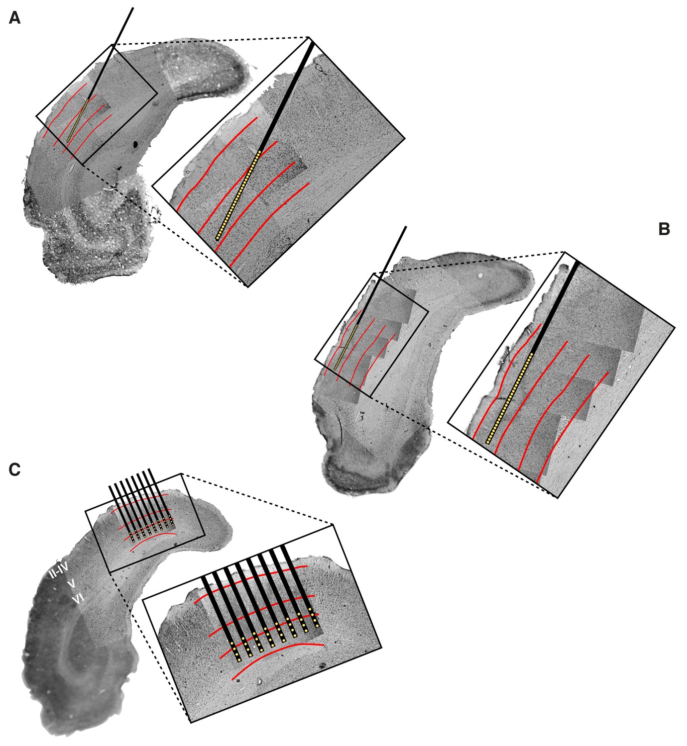
Histological reconstruction of the laminar location of the recording sites.
Histological reconstruction of the recording sites for three example experimental sessions, two targeting lateral extrastriate areas LM, LI and LL (A–B) and one targeting primary visual cortex (C). The recordings were performed with different configurations of 32-channel silicon probes. In (A–B), a single-shank probe (model A1 × 32-5mm50-413), with recording sites spanning 1550 µm, was inserted diagonally into rat visual cortex, in such a way to target either the deep (A) or superficial (B) layers of areas LM, LI and LL. Note that the histological section shown in (A) refers to the same section shown in Figure 1A. In (C), an 8-shank probe (model A8 × 4-2mm100-200-177), with recording sites spanning an area of 1400 µm (across shanks) x 300 µm (within shank), was inserted perpendicularly into primary visual cortex (V1), targeting deep layers. Each panel shows a low magnification image of the Nissl-stained coronal section at the targeted bregma, with superimposed higher-magnification Nissl images (either 2.5X or 10X), taken around the insertion track(s) of the probe. These images were stitched together to obtain a high-resolution picture of the probe location, with respect to the cortical layers. The position of the recording sites was reconstructed by tracing the outline of the fluorescent track left by each shank (that had been coated with the fluorescent dye DiI before insertion; e.g., see the red trace in Figure 1A), and then relying on the known geometry of the probe (see Materials and methods for details). The resulting position of the shank(s) and recording sites are indicated, respectively, by the thick black lines and by the yellow dots. The red lines show the boundaries between different groups of cortical laminae: layers II-IV, layer V and layer VI. These boundaries were estimated from the variation of cell size, morphology and density across the cortical thickness.
Figure 1—figure supplement 2
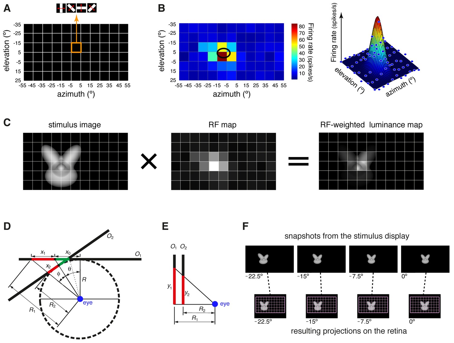
Computation of the receptive field size and receptive field luminance, and illustration of the tangent screen projection.
(A) Illustration of the virtual grid of 6 × 11, 10°-wide cells, where the drifting bars used to map the neuronal receptive fields (RFs) were shown. In each cell, the bars were presented at four different orientations (0°, 45°, 90° and 135°), sweeping from one side of the cell to the opposite one and back at the speed of 66°/s. (B) Receptive field map (left), resulting from plotting the average number of spikes fired by a neuron, in response to the four oriented bars, across the grid of visual field locations shown in (A). In the right plot, the same firing intensity map is rendered in three dimensions (blue dots), along with the two-dimensional Gaussian (mesh grid surface) that best fitted the data points. The ellipse centered on the peak of the Gaussian and defined by its widths along the x and y axes was taken as the extent of the neuronal RF (black ellipse in the left plot). (C) Illustration of the procedure to compute the RF luminance of a visual stimulus. The image of an example visual stimulus (left plot) is superimposed to the grid used to map the RF of a recorded neuron (middle plot; same RF as in B). The two maps (i.e., the stimulus image and the RF) are multiplied in a cell-by-cell fashion, so as to yield an RF-weighted luminance intensity map of the stimulus (right plot). These luminance intensity values are then summed to obtain the RF luminance of the stimulus (this procedure is equivalent to compute the dot product between the stimulus image and the RF map). The standard deviation of the RF-weighted luminance intensity values falling inside the RF was taken as a measure of the contrast impinged by the stimulus on the RF (we called this metric RF contrast; see Materials and methods). Note that, in (A–C), the lines of the grid are shown only to help visualizing the spatial arrangement and extent of the stimuli and of the RF map, but no grid was actually shown during stimulus presentation. (D–E) Illustration of the tangent screen projection used to present the visual stimuli in our experiment. This projection avoided distorting the shape of the objects, when they were translated across the stimulus display, in spite of the close proximity of the eye to the display. See Materials and methods for a detailed explanation of the variables and their relationship. (F) The images in the top row are snapshots taken from the stimulus display during the presentation of an example object at four different azimuth locations (−22.5°, −15°, −7.5° and 0°). It can be noticed the distortion applied to the object by the tangent screen projection to compensate for the distortion produced by the perspective projection to the retina. The bottom row shows the resulting projections of the object over the retina. To provide a spatial reference, the grid of visual field locations used to map the neuronal RFs is also shown (pink grid).
Figure 2 with 1 supplement
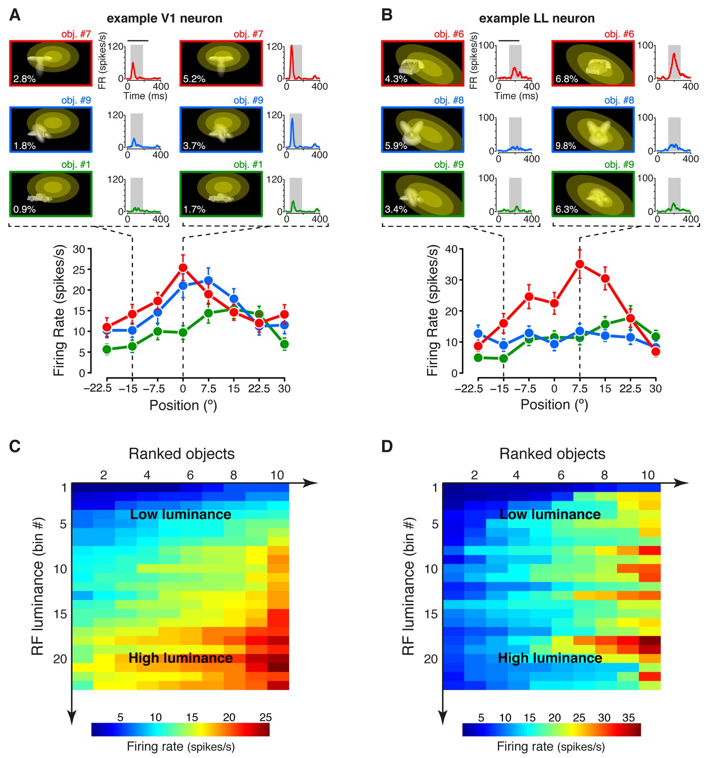
Tuning of an example V1 and LL neuron.
(A–B) The bottom plots show the average firing rates (AFRs) of a V1 (A) and a LL (B) neuron, evoked by three objects, presented at eight different visual field positions (shown in Figure 1B.1). The top plots show the peri-stimulus time histograms (PSTHs) obtained at two positions, along with the images of the corresponding stimulus conditions. These images also display the RF profile of each neuron, in the guise of three concentric ellipses, corresponding to 1 SD, 2 SD and 3 SD of the two-dimensional Gaussians that were fitted to the raw RFs. The numbers (white font) show the luminosity that each object condition impinged on the RF (referred to as RF luminance; the distributions of RF luminance values produced by the objects across the full set of positions and the full set of transformations are shown in Figure 2—figure supplement 1). The gray patches over the PSTHs show the spike count windows (150 ms) used to compute the AFRs (their onsets were the response latencies of the neurons). Error bars are SEM. (C–D) Luminance sensitivity profiles for the two examples neurons shown in (A) and (B). For each neuron, the stimulus conditions were grouped in 23 RF luminance bins with 10 stimuli each, and the intensity of firing across the resulting 23 × 10 matrix was color-coded. Within each bin, the stimuli were ranked according to the magnitude of the response they evoked.
Figure 2—figure supplement 1
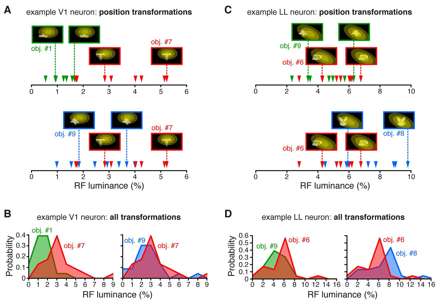
RF luminance values produced by very effective and poorly effective objects: a comparison between an example V1 and an example LL neuron.
(A) The arrows show the RF luminance values that were measured, across eight positions, for three objects that were differently effective at driving an example V1 neuron (same cell of Figure 2A and C). The most effective object (#7; see Figure 2A) consistently yielded larger RF luminance values (red arrows), compared to the least effective one (#1; green arrows). By comparison, another object (#9), which was also quite effective at driving the cell (see Figure 2A), produced RF luminance values (blue arrows) that substantially overlapped with those of object #7. (B) Same comparison as in (A), but with the distributions of RF luminance values of the three objects, computed across the full set of 23 transformations each object underwent (same color code as in A). (C) The RF luminance values produced by three objects, across eight positions, for an example LL neuron (same cell of Figure 2B and D). In this case, the most effective object (#6; see Figure 2B) did not yield the largest RF luminance values (red arrows). The other two objects (#9 and #8), which were both ineffective at driving the cell (see Figure 2B), produced either very similar (#9; green arrows) or considerably larger (#8; blue arrows) RF luminance values, as compared to object #6. (D) Same comparison as in (C), but with the distributions of RF luminance values of the three objects, computed across the full set of 23 transformations each object underwent (same color code as in C).
Figure 3 with 4 supplements
Information conveyed by the neuronal response about stimulus luminance and luminance-independent visual features.
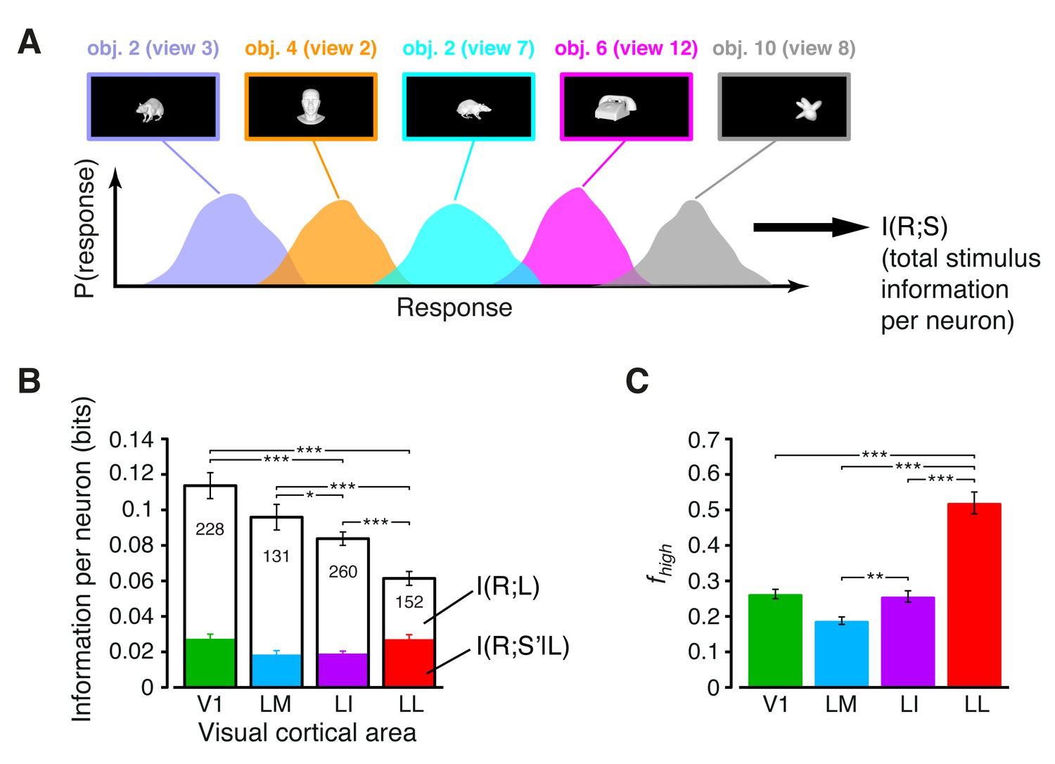
(A) Illustration of how total stimulus information per neuron was computed. All the views of all the objects (total of 230 stimuli) were considered as different stimulus conditions, each giving rise to its own response distribution (colored curves; only a few examples are shown here). Mutual information between stimulus and response measured the discriminability of the stimuli, given the overlap of their response distributions. (B) Mutual information (median over the units recorded in each area ± SE) between stimulus and response in each visual area (full bars; *p<0.05, **p<0.01, ***p<0.001; 1-tailed U-test, Holm-Bonferroni corrected). The white portion of the bars shows the median information that each area carried about stimulus luminance, while the colored portion is the median information about higher-order, luminance-independent visual features. The number of cells in each area is written on the corresponding bar. (C) Median fraction of luminance-independent stimulus information (; see Results) that neurons carried in each area. Error bars and significance levels/test as in (B). The mutual information metrics obtained for neurons sampled from cortical layers II-IV and V-VI are reported in Figure 3—figure supplement 1. The values obtained for neuronal subpopulations with matched spike isolation quality are shown in Figure 3—figure supplement 2. The sensitivity of rat visual neurons to luminance variations of the same object is shown in Figure 3—figure supplement 3. The information carried by rat visual neurons about stimulus contrast and contrast-independent visual features is reported in Figure 3—figure supplement 4.
Figure 3—figure supplement 1
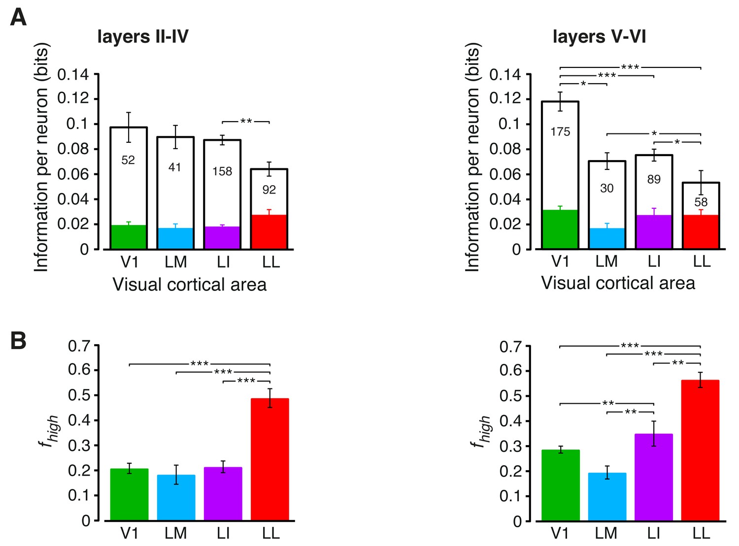
Information conveyed by the neuronal response about stimulus luminance and luminance-independent visual features: a comparison between superficial and deep layers.
Same mutual information analysis as the one shown in Figure 3, but considering separately the neuronal populations recorded in cortical layers II-IV (left plots) and V-VI (right plots). Colors, symbols, significance levels and statistical tests as in Figure 3. (A) To check whether the drop of stimulus information (full bars) was similarly sharp in superficial and deep layers, a two-way ANOVA, with visual area and layer as factors, was carried out. The test yielded a significant main effect for area (p<0.001, F3,687 = 15.87) and a significant interaction between area and layer (p<0.001, F3,687 = 5.61), but not a main effect for layer alone (p>0.9, F1,687 = 0.01). This indicates that the information loss was sharper in deep layers. As for the case of the entire populations (see Figure 3B), the drop of information was mainly due to a reduction of the information about stimulus luminosity (white bars), while the information about higher-order visual attributes (colored bars) remained more stable across the areas. This was especially noticeable for deep layers, where the information about luminosity in LM and LI became almost half as large as in V1, further dropping in LL to about one third of what observed in V1. (B) The fraction of luminance-independent stimulus information (fhigh) that neurons carried in each area increased more gradually and was, overall, larger in deep than in superficial layers. A two-way ANOVA, with visual area and layer as factors, confirmed this observation, yielding a significant main effect for both area (p<0.001, F3,687 = 63.58) and layer (p<0.001, F1,687 = 14.7) and also a significant interaction (p<0.01, F3,687 = 4.06). In terms of pairwise comparisons, this resulted in a very large and significant increase of fhigh in LL, as compared to all other areas, in both superficial and deep layers, and in a significant difference also between LI and V1/LM, but in deep layers only.
Figure 3—figure supplement 2
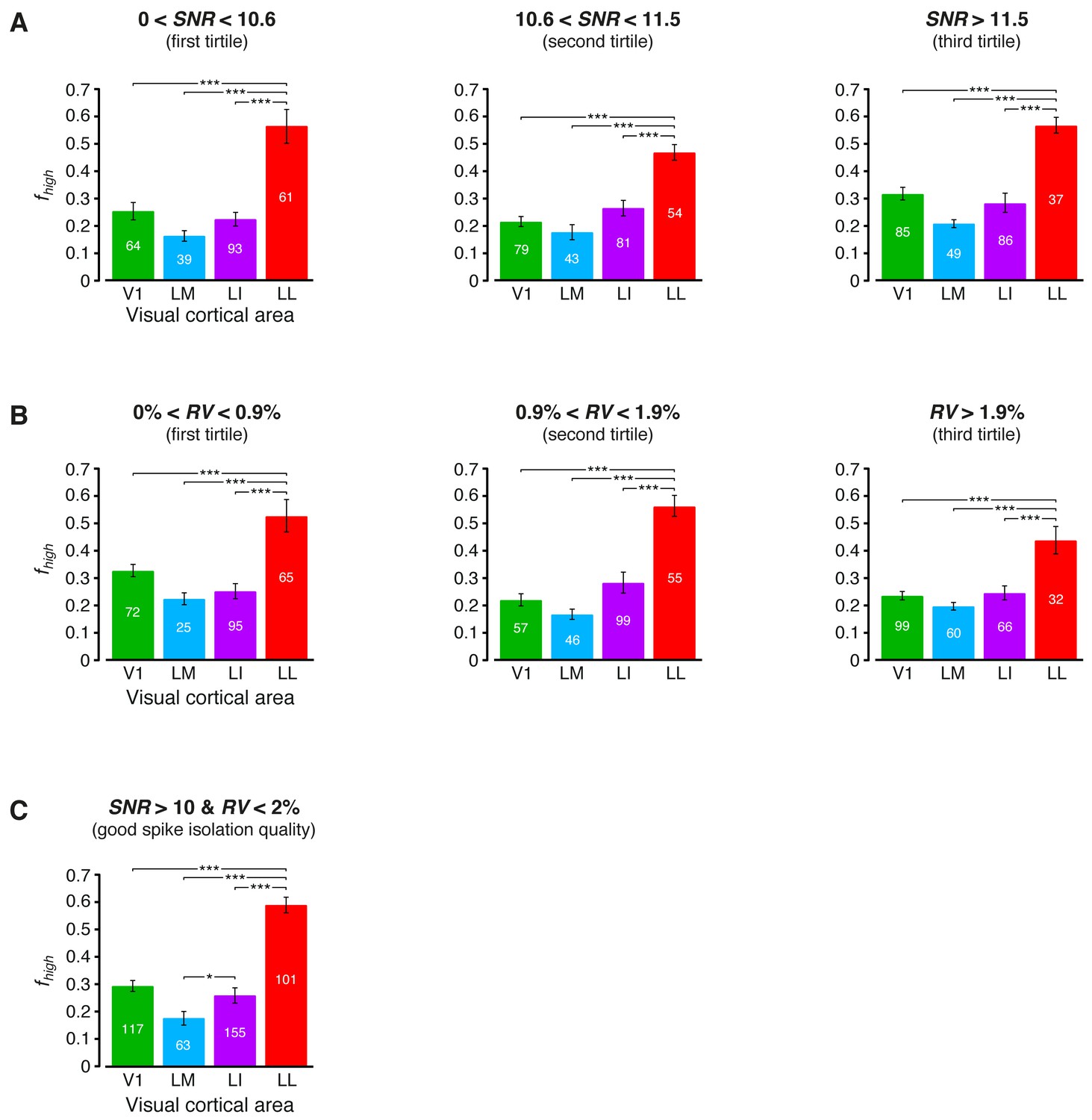
Independence of the fraction of luminance-independent stimulus information from the quality of spike isolation.
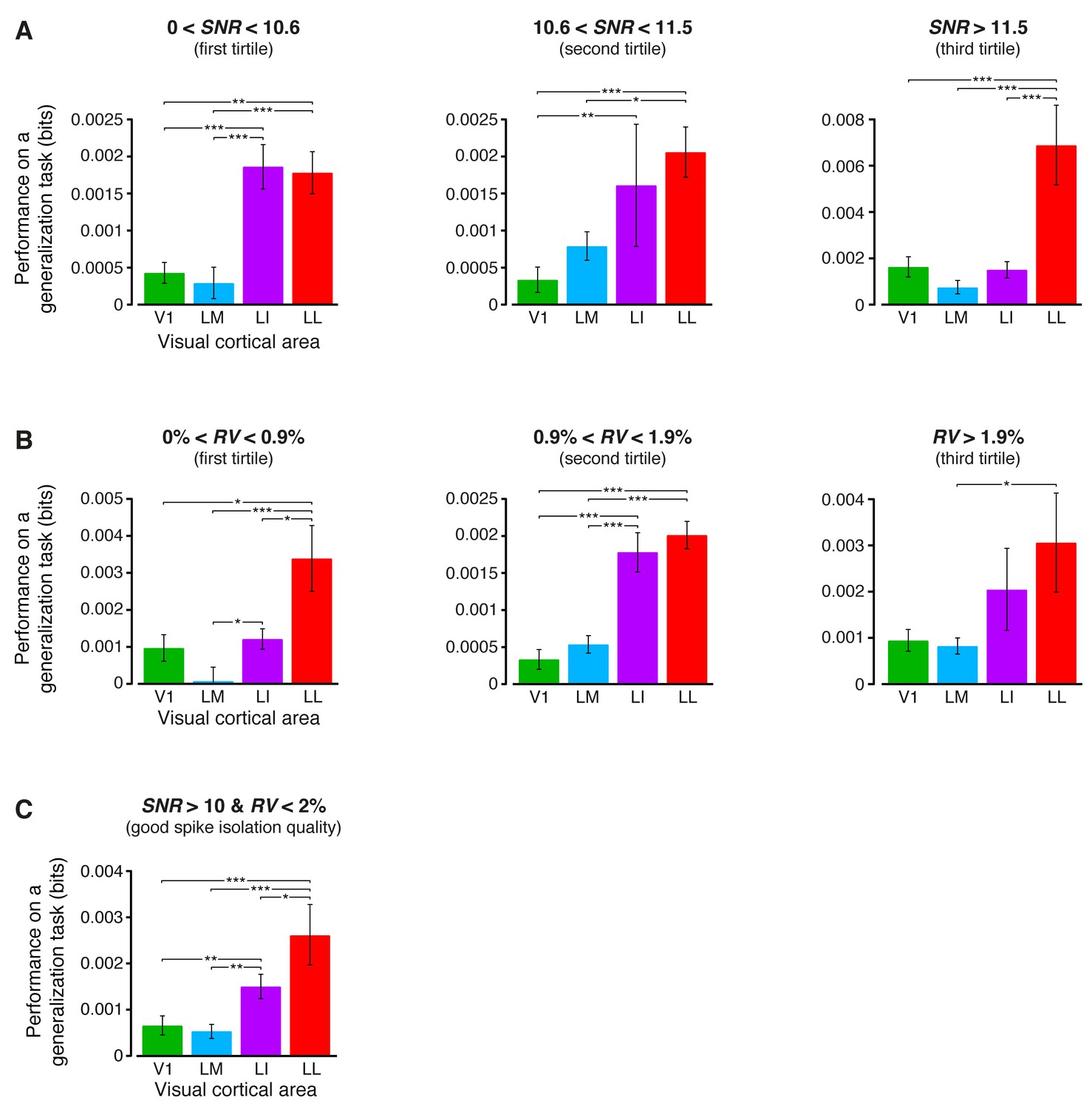
(A–B) Same mutual information analysis as the one shown in Figure 3C, but restricted to units within a given tirtile of the SNR and RV metrics, used to asses the quality of spike isolation (see Materials and methods). Note that the quality of spike isolation increases as function of SNR, while it decreases as a function of RV. The number of units in each area per tirtile is superimposed to the corresponding bar. (C) Same mutual information analysis, considering only the neuronal subpopulations with good spike isolation quality (i.e., with both SNR >10 and RV <2%) – these constraints also equated the neuronal subpopulations in terms of firing rate (Figure 6—figure supplement 3B). In (A–C), symbols, significance levels, and statistical tests are as in Figure 3.
Figure 3—figure supplement 3

Sensitivity of rat visual neurons to luminance variations of the same object.
(A) The thin black curves show the sensitivity to luminance variations of the same object for the neurons recorded in each area. Each curve was obtained by taking, for each neuron, the responses across the four luminance levels that were tested for each object (i.e., 12.5%, 25%, 50% and full luminance; see the example images reported below the abscissa in the leftmost panel), and then averaging these responses across the 10 object identities. This yielded a curve showing the average response of the neuron to each luminance level. Each curve was then normalized to its maximum, so as to allow a better comparison among the different neurons in a given area. The colored curves show the averages of these luminance-sensitivity curves across all the neurons recorded in each area. Note that the luminance levels on the abscissa are reported on a logarithmic scale. (B) For each neuron, the sharpness of its sensitivity to luminance changes of the same object was quantified by computing the sparseness of the black curves shown in (A). The bars show how the sparseness decreased across the four visual areas (median over the units recorded in each area ± SE; **p<0.01, 1-tailed U-test, Holm-Bonferroni corrected).
Figure 3—figure supplement 4

Information conveyed by the neuronal response about stimulus contrast and contrast-independent visual features.
(A) The full bars show the mutual information (median over the units recorded in each area ± SE) between stimulus and response in each visual area. The white portion of the bars shows , the information that each area carried about stimulus contrast C (as measured by the RF contrast metric; see Materials and methods), while the colored portion shows , the information about stimulus identity (S’), as defined by any possible visual attribute with the exception of the RF contrast. The number of cells in each area is written on the corresponding bar. Note these numbers are lower than the total numbers of neurons recorded in each area (e.g., compare to Figure 3B), because only a fraction of units met the criterion to be included in this analysis (see Materials and methods). Also note that, because only a subset of neurons and object conditions contributed to this analysis (see Materials and methods), the total stimulus information reported here for V1, LM and LI is lower than the total stimulus information shown in Figure 3B. In particular, this is due to the fact that only stimuli that covered at least 10% of each RF were included in this analysis (see Materials and methods). This reduced the range of luminance values spanned by the stimulus conditions – a fact that, given the strong luminance sensitivity of V1, LM and LI neurons (see Figure 3B), produced the drop of stimulus information carried by individual neurons in these areas. No appreciable reduction of total stimulus information was found in LL (compare the fourth full bar in this figure to the matching bar in Figure 3B), thus confirming once more the much lower sensitive of LL neurons to stimulus luminance. (B) Median fraction of contrast-independent stimulus information that neurons carried in each area. Error bars are SEs of the medians (*p<0.05, **p<0.01, ***p<0.001; 1-tailed U-test, Holm-Bonferroni corrected).
Figure 4 with 1 supplement

Comparing total visual information and view-invariant object information per neuron.
(A) Illustration of how total visual information and view-invariant object information per neuron were computed, given an object pair. In the first case, all the views of the two objects were considered as different stimulus conditions, each giving rise to its own response distribution (colored curves). In the second case, the response distributions produced by different views of the same object were merged into a single, overall distribution (shown in blue and red, respectively, for the two objects). (B) Total visual information per neuron (median over the units recorded in each area ± SE) as a function of the similarity between the RF luminance of the objects in each pair, as defined by (see Results). (C) Left: view-invariant object information per neuron (median ± SE) as a function of . Right: view-invariant object information per neuron (median ± SE) for (*p<0.05, **p<0.01, ***p<0.001; 1-tailed U-test, Holm-Bonferroni corrected). The number of cells in each area is written on the corresponding bar. (D) Ratio between view-invariant object information and total information per neuron (median ± SE), for . Significance levels/test as in (C). The invariant object information carried by RF luminance as a function of is reported in Figure 4—figure supplement 1.
Figure 4—figure supplement 1
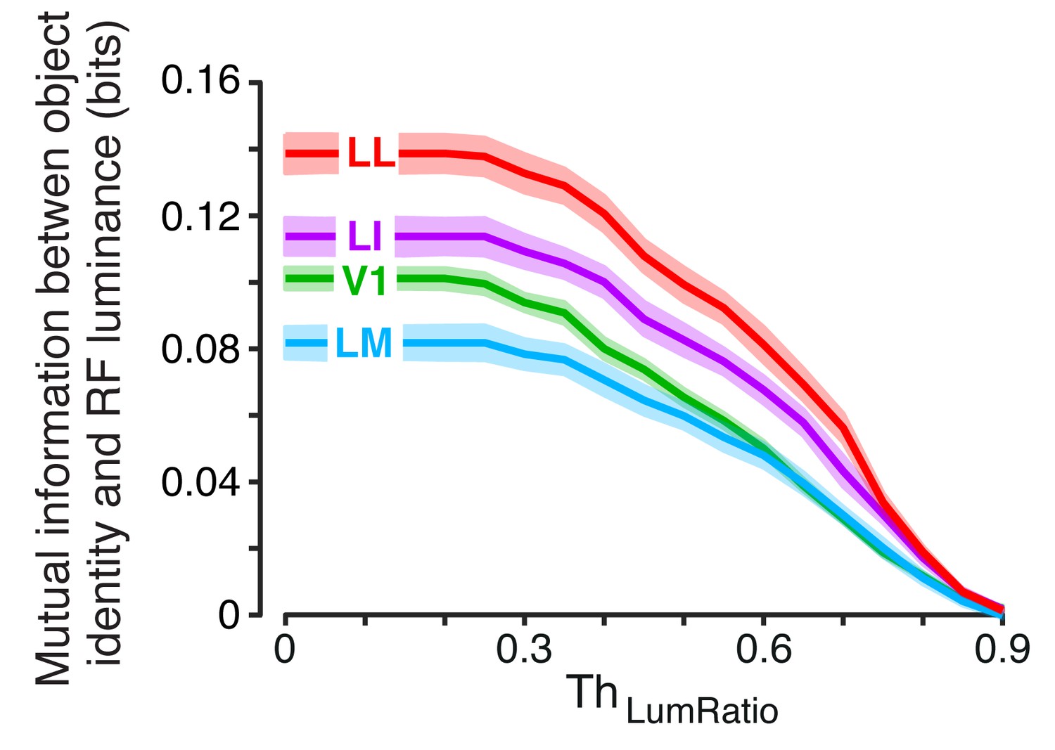
Invariant object information carried by RF luminance as a function of .
For each neuron and object pair, we computed , the mutual information between object identity (with all the views of each object in the pair taken into account) and RF luminance. The colored curves show the median of (± SE) across all the units recorded in each area as a function of the similarity between the RF luminance of the objects in each pair, as defined by (see Results).
Figure 5
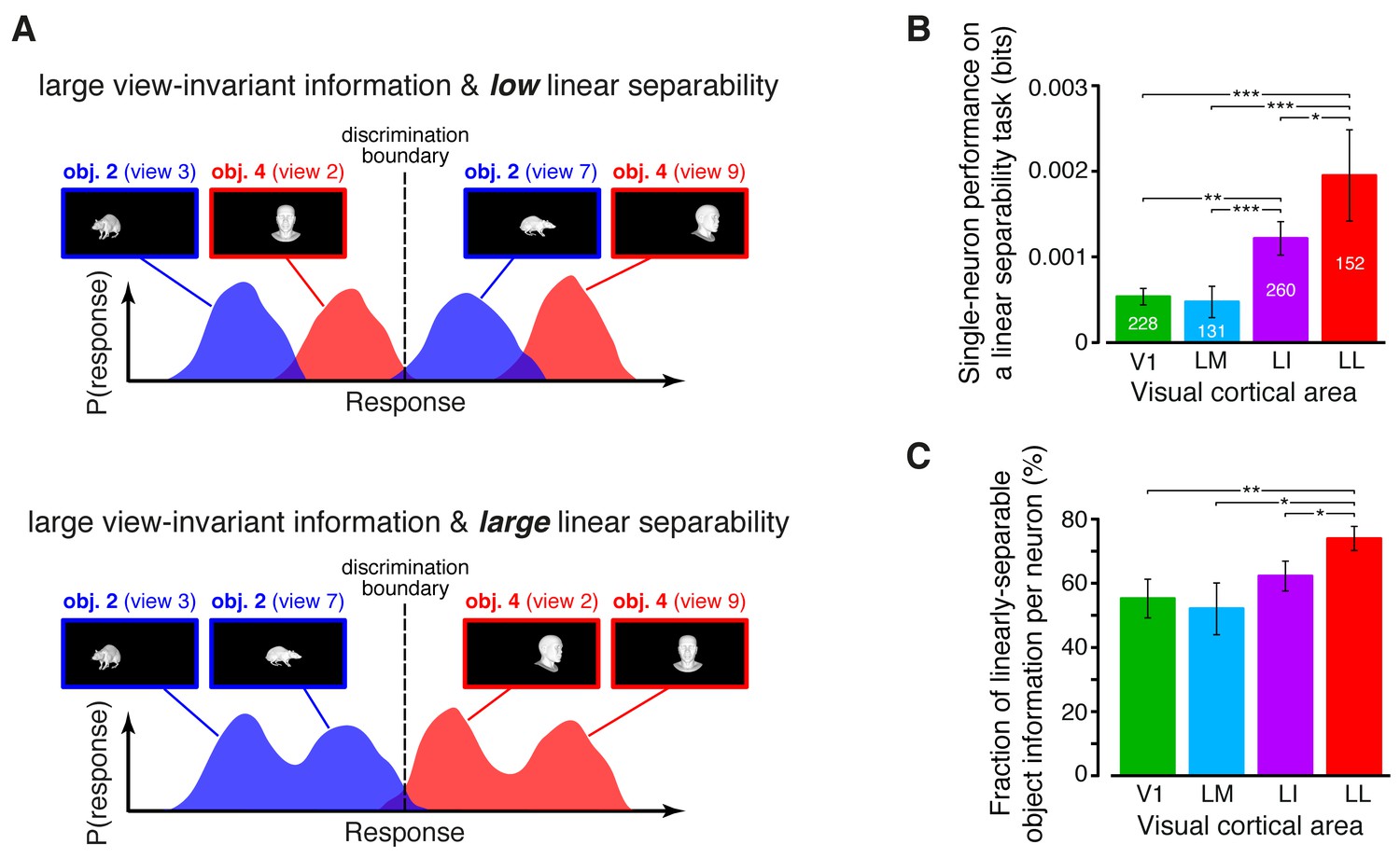
Linear separability of object representations at the single-neuron level.
(A) Illustration of how a similar amount of view-invariant information per neuron can be encoded by object representations with a different degree of linear separability. The overlap between the response distributions produced by two objects across multiple views is similarly small in the top and bottom examples; hence, the view-invariant object information per neuron is similarly large. However, only for the distributions shown at the bottom, a single discrimination boundary can be found (dashed line) that allows discriminating the objects regardless of their specific view. (B) Linear separability of object representations at the single-neuron level (median over the units recorded in each area ± SE; *p<0.05, **p<0.01, ***p<0.001; 1-tailed U-test, Holm-Bonferroni corrected). The number of cells in each area is written on the corresponding bar. (C) Ratio between linear separability, as computed in (B), and view-invariant object information, as computed in Figure 4C, right (median ± SE). Significance levels/test as in (B). In both (B) and (C), .
Figure 6 with 3 supplements
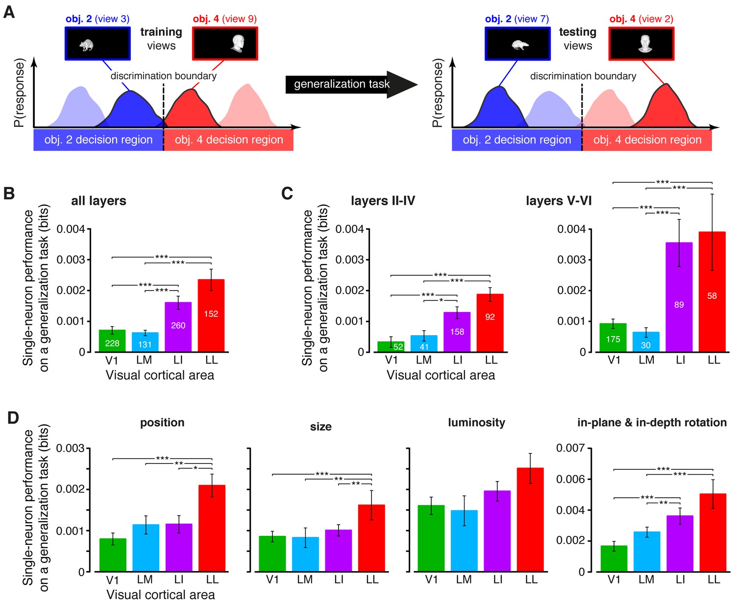
Ability of single neurons to support generalization to novel object views.
(A) Illustration of how the ability of single neurons to discriminate novel views of previously trained objects was assessed. The blue and red curves refer to the hypothetical response distributions evoked by different views of two objects. A binary decoder is trained to discriminate two specific views (darker curves, left), and then tested for its ability to correctly recognize two different views (darker curves, right), using the previously learned discrimination boundary (dashed lines). (B) Generalization performance achieved by single neurons with novel object views (median over the units recorded in each area ± SE; *p<0.05, **p<0.01, ***p<0.001; 1-tailed U-test, Holm-Bonferroni corrected). The number of cells in each area is written on the corresponding bar. (C) Median generalization performances (± SE) achieved by single neurons for the neuronal subpopulations sampled from cortical layers II-IV (left) and V-VI (right). Significance levels/test as in (B). Note that the laminar location was not retrieved for all the recorded units (see Materials and methods). (D) Median generalization performances (± SE) achieved by single neurons, computed along individual transformation axes. In (C–D), significance levels/test are as in (B). in (B–D). The generalization performances achieved by single neurons across parametric position and size changes are reported in Figure 6—figure supplement 1. The generalization performances obtained for neuronal subpopulations with matched spike isolation quality are shown in Figure 6—figure supplement 2. The firing rate magnitude measured in the four areas (before and after matching the neuronal populations in terms of spike isolation quality) is reported in Figure 6—figure supplement 3.
Figure 6—figure supplement 1
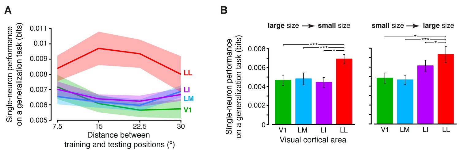
Generalization achieved by single neurons across parametric position and size changes.
(A) The curves show the generalization performances of binary decoders (median over the units recorded in each area ± SE) that were trained to discriminate two objects presented at the same position in the visual field, and then were required to discriminate those same objects across increasingly wider positions changes, with respect to the training location (see Materials and methods for details). Differences among the four areas were quantified by a two-way ANOVA with visual area and distance from the training position as factors. The main effects of area (F3,595 = 4.078) and distance (F3,1785 = 2.706) were both significant (p<0.01 and p<0.05, respectively), thus confirming the existence of a gradient in the amount of position tolerance along the areas’ progression and along the distance axis. The interaction term was also significant (p<0.001, F9,1785 = 3.239), indicating that the four decoding performances dropped at a different pace along the distance axis. (B) Discrimination performances of binary decoders (median over the units recorded in each area ± SE) that were required to generalize from a given training size to either a smaller (left) or larger (right) test size (see Materials and methods for details; *p<0.05, **p<0.01, ***p<0.001; 1-tailed U-test, Holm-Bonferroni corrected).
Figure 6—figure supplement 2
Independence of the generalization performances yielded by single neurons from the quality of spike isolation.
(A–B) Same decoding analysis as the one shown in Figure 6B, but restricted to units within a given tirtile of the SNR and RV metrics, used to asses the quality of spike isolation (see Materials and methods and the legend of Figure 3—figure supplement 2). The number of units in each area per tirtile is the same reported in Figure 3—figure supplement 2A–B. (C) Same decoding analysis, considering only the neuronal subpopulations with good spike isolation quality (i.e., with both SNR >10 and RV <2%) – these constraints also equated the neuronal subpopulations in terms of firing rate (Figure 6—figure supplement 3B). In (A–C), symbols, significance levels, and statistical tests are as in Figure 6B.
Figure 6—figure supplement 3
Magnitude of the firing rates.
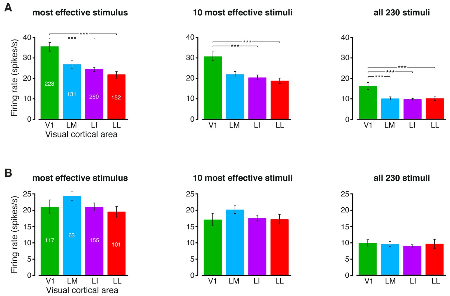
(A) Median number of spikes per second fired by the neurons in each visual area, as a response to: (1) the most effective object condition (left); (2) the 10 most effective object conditions (middle); and (3) all the 230 object conditions used in the single-cell information theoretic and decoding analyses. Error bars are SE of the medians. Stars indicate the statistical significance of pairwise comparisons (*p<0.05, **p<0.01, ***p<0.001; 1-tailed U-test, Holm-Bonferroni corrected). The number of cells in each area is superimposed to the corresponding bar. (B) Same plots as in (A), but after considering only the neuronal subpopulations with good spike isolation quality (i.e., same subpopulations as in Figure 3—figure supplement 2C and Figure 6—figure supplement 2C). As a result of this selection, the median firing rates became statistically indistinguishable across all the four visual areas.
Figure 7 with 1 supplement
Single-neuron decoding and mutual information metrics, compared across neuronal subpopulations with matched RF size.
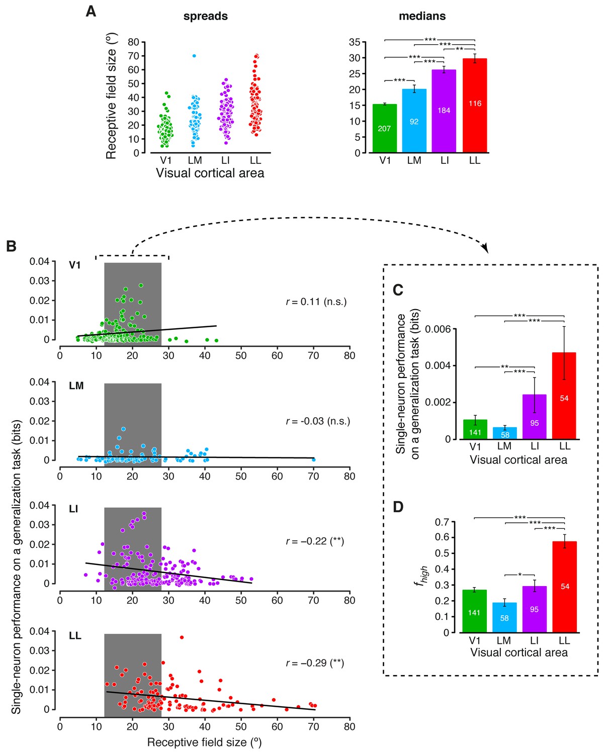
(A) Spreads (left) and medians ± SE (right) of the RF sizes measured in each visual area (*p<0.05, **p<0.01, ***p<0.001; 1-tailed U-test, Holm-Bonferroni corrected). The number of cells in each area for which RF size could be estimated is reported on the corresponding bar of the right chart. Spreads and medians of the response latencies are reported in Figure 7—figure supplement 1. (B) For each visual area, the generalization performances achieved by single neurons (same data of Figure 6B) are plotted against the RF sizes (same data of panel A). In the case of LI and LL, these two metrics were significantly anti-correlated (**p<0.01; 2-tailed t-test). (C) Median generalization performances (± SE) achieved by single neurons, as in Figure 6B, but considering only neuronal subpopulations with matched RF size ranges, indicated by the gray patches in (B) (*p<0.05, **p<0.01, ***p<0.001; 1-tailed U-test, Holm-Bonferroni corrected). The number of neurons in each area fulfilling this constraint is reported on the corresponding bar. (D) Median fraction of luminance-independent stimulus information (± SE) conveyed by neuronal firing as in Figure 3C, but including only the RF-matched subpopulations used in (C). Significance levels/test as in (C).
Figure 7—figure supplement 1
Response latencies.
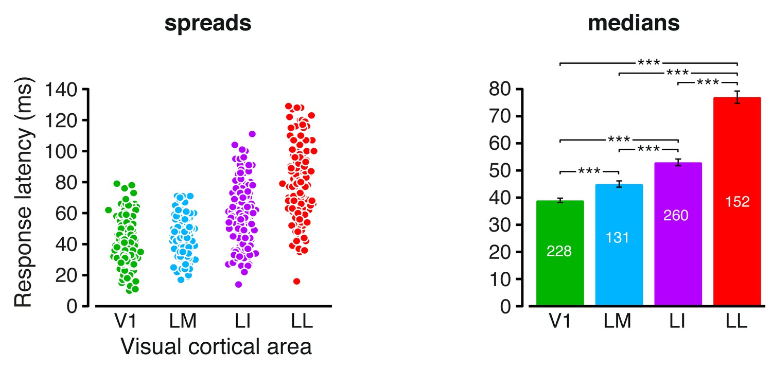
Spreads (left) and medians ± SE (right) of the response latencies measured in each visual area (*p<0.05, **p<0.01, ***p<0.001; 1-tailed U-test, Holm-Bonferroni corrected). The number of cells in each area is reported on the corresponding bar of the right chart.
Figure 8 with 3 supplements
Linear separability and generalization of object representations, tested at the level of neuronal populations.
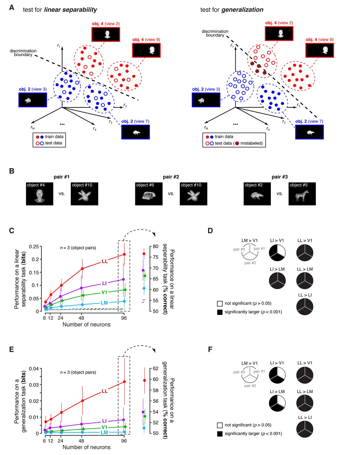
(A) Illustration of the population decoding analyses used to test linear separability and generalization. The clouds of dots show the sets of response population vectors produced by different views of two objects. Left: for the test of linear separability, a binary linear decoder is trained with a fraction of the response vectors (filled dots) to all the views of both objects, and then tested with the left-out response vectors (empty dots), using the previously learned discrimination boundary (dashed line). The cartoon depicts the ideal case of two object representations that are perfectly separable. Right: for the test of generalization, a binary linear decoder is trained with all the response vectors (filled dots) produced by a single view per object, and then tested for its ability to correctly discriminate the response vectors (empty dots) produced by the other views, using the previously learned discrimination boundary (dashed line). As illustrated here, perfect linearly separability does not guarantee perfect generalization to untrained object views (see the black-filled, mislabeled response vectors in the right panel). (B) The three pairs of visual objects that were selected for the population decoding analyses shown in C-F, based on the fact that their luminance ratio fulfilled the constraint of being larger than for at least 96 neurons in each area. (C) Classification performance of the binary linear decoders in the test for linear separability, as a function of the number of neurons N used to build the population vector space. Performances were computed for the three pairs of objects shown in (B). Each dot shows the mean of the performances obtained for the three pairs (± SE). The performances are reported as the mutual information between the actual and the predicted object labels (left). In addition, for N = 96, they are also shown in terms of classification accuracy (right). The dashed lines (left) and the horizontal marks (right) show the linear separability of arbitrary groups of views of two objects (same three pairs used in the main analysis; see Results). (D) The statistical significance of each pairwise area comparison, in terms of linear separability, is reported for each individual object pair (1-tailed U-test, Holm-Bonferroni corrected). In the pie charts, a black slice indicates that the test was significant (p<0.001) for the corresponding pairs of objects and areas (e.g., LL > LI). (E) Classification performance of the binary linear decoders in the test for generalization across transformations. Same description as in (C). (F) Statistical significance of each pairwise area comparison, in terms of generalization across transformations. Same description as in (D). The same analyses, performed over a larger set of object pairs, after setting , are shown in Figure 8—figure supplement 1. The dependence of linear separability and generalization from is shown in Figure 8—figure supplement 2. The statistical comparison between the performances achieved by a population of 48 LL neurons and V1, LM and LI populations of 96 neurons is reported in Figure 8—figure supplement 3.
Figure 8—figure supplement 1
Linear separability and generalization of object representations, tested at the level of neuronal populations, using a larger set of object pairs.
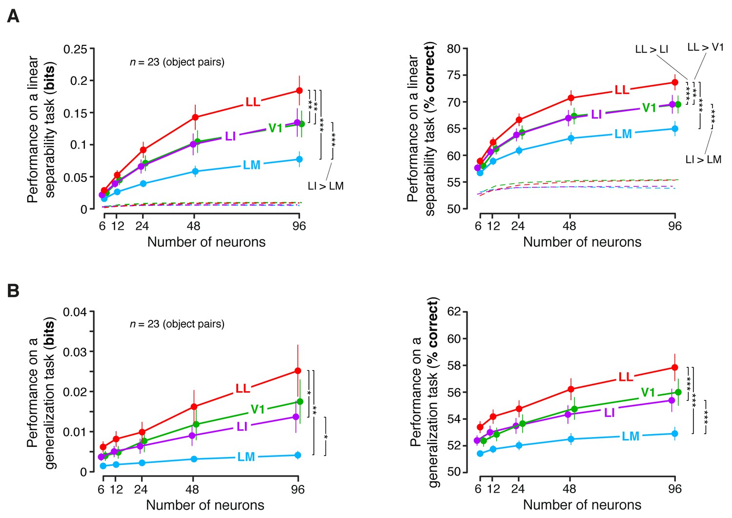
(A) Classification performance of binary linear decoders in the test for linear separability (see Figure 8A, left), as a function of the size of the neuronal subpopulations used to build the population vector space. This plot is equivalent to the one shown in Figure 8C, with the difference that, here, the objects that the decoders had to discriminate were allowed to differ more in terms of luminosity (this was achieved by setting ). As a result, much more object pairs (23) could be tested, compared to the analysis shown in Figure 8C. Each dot shows the mean of the 23 performances obtained for these object pairs and the error bar shows its SE. The larger number of object pairs allowed applying a 1-tailed, paired t-test (with Holm-Bonferroni correction) to assess whether the differences among the average performances in the four areas were statistically significant (*p<0.05, **p<0.01, ***p<0.001). The performances are reported both as mutual information between actual and predicted object labels (left) and as classification accuracy (i.e., as the percentage of correctly labeled response vectors; right). (B) Classification performance of binary linear decoders in the test for generalization across transformations (see Figure 8A, right). Same description as in (A).
Figure 8—figure supplement 2
Dependence of linear separability and generalization, measured at the neuronal population level, from the luminance difference of the objects to discriminate.
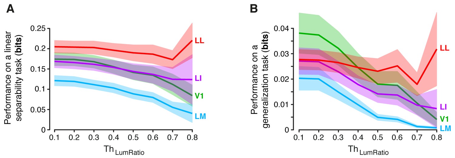
(A) Classification performance of binary linear decoders in the test for linear separability (see Figure 8A, left) as a function of the similarity between the RF luminance of the objects to discriminate, as defined by (see Results). The curves, which were produced using populations of 96 neurons, report the median performance in each visual area (± SE) over all the object pairs obtained for a given value of . Note that, for and , the performances are equivalent to those already shown in the left panels Figure 8C and Figure 8—figure supplement 1A (rightmost points). Also note that, for , all the available object pairs contributed to the analysis. As such, the corresponding performances are those yielded by the four visual areas when no restriction was applied to the luminosity of the objects to discriminate. (B) Same analysis as in (A), but for the test of generalization across transformations (see Figure 8A, right).
Figure 8—figure supplement 3

Statistical comparison between the performance achieved by a population of 48 LL neurons and the performances yielded by populations of 96 neurons in V1, LM and LI.
(A) For each of the three object pairs tested in Figure 8 (shown in Figure 8B), we checked whether a population of 48 LL neurons yielded a significantly larger performance than V1, LM and LI populations of twice the number of neurons (i.e., 96 units) in the linear discriminability task (see Figure 8A, left). The resulting pie chart shown here should be compared to the rightmost column of the pie chart in Figure 8D, with a black slice indicating that the comparison was significant (p<0.001; 1-tailed U-test, Holm-Bonferroni corrected) for the corresponding pairs of objects and areas – e.g., LL (48 units) > LI (96 units). (B) Same analysis as in (A), but for the test of generalization across transformations (see Figure 8A, right). The pie chart shown here should be compared to the rightmost column of the pie chart in Figure 8F.
Download links
A two-part list of links to download the article, or parts of the article, in various formats.
Downloads (link to download the article as PDF)
Open citations (links to open the citations from this article in various online reference manager services)
Cite this article (links to download the citations from this article in formats compatible with various reference manager tools)
Emergence of transformation-tolerant representations of visual objects in rat lateral extrastriate cortex
eLife 6:e22794.
https://doi.org/10.7554/eLife.22794


