Using the Volta phase plate with defocus for cryo-EM single particle analysis
- Max Planck Institute of Biochemistry, Germany
- Max Planck Institute for Biophysical Chemistry, Germany
Figures
Figure 1
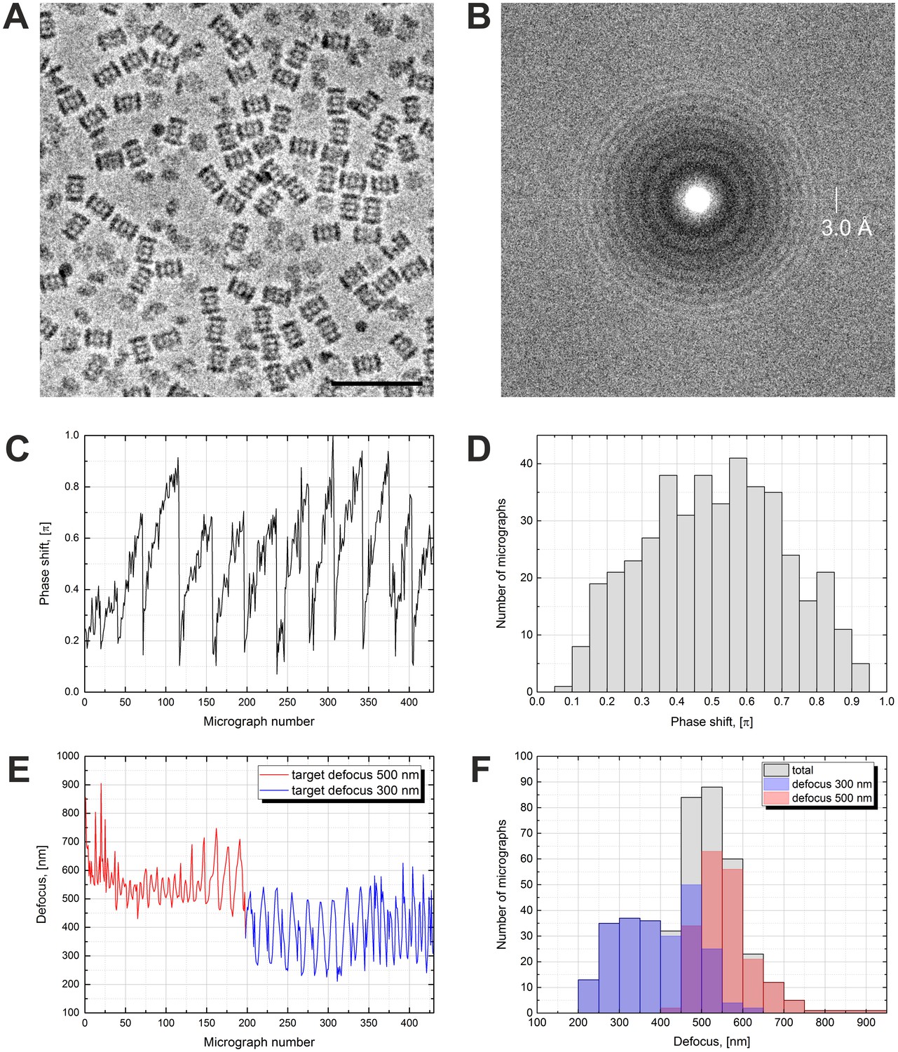
Volta phase plate with defocus cryo-EM dataset of 20S proteasome.
(A) Representative image of 20S proteasomes in ice, defocus 500 nm. (B) Power spectrum of the image in (A) showing contrast transfer function rings (Thon rings). To enhance the visibility of Thon rings, the power spectrum was calculated as the sum of the power spectra of individual movie frames (McMullan et al., 2015). (C) Phase shift history throughout the dataset. The phase shift gradually increases until the phase plate is moved to a new position where it suddenly drops and starts to raise again. (D) Histogram illustrating the phase shift distribution. (E) Defocus history throughout the dataset. The target defocus was changed after ~200 images from 500 nm to 300 nm. (F) Histograms illustrating the defocus distributions. Scale bar: 50 nm.
Figure 2
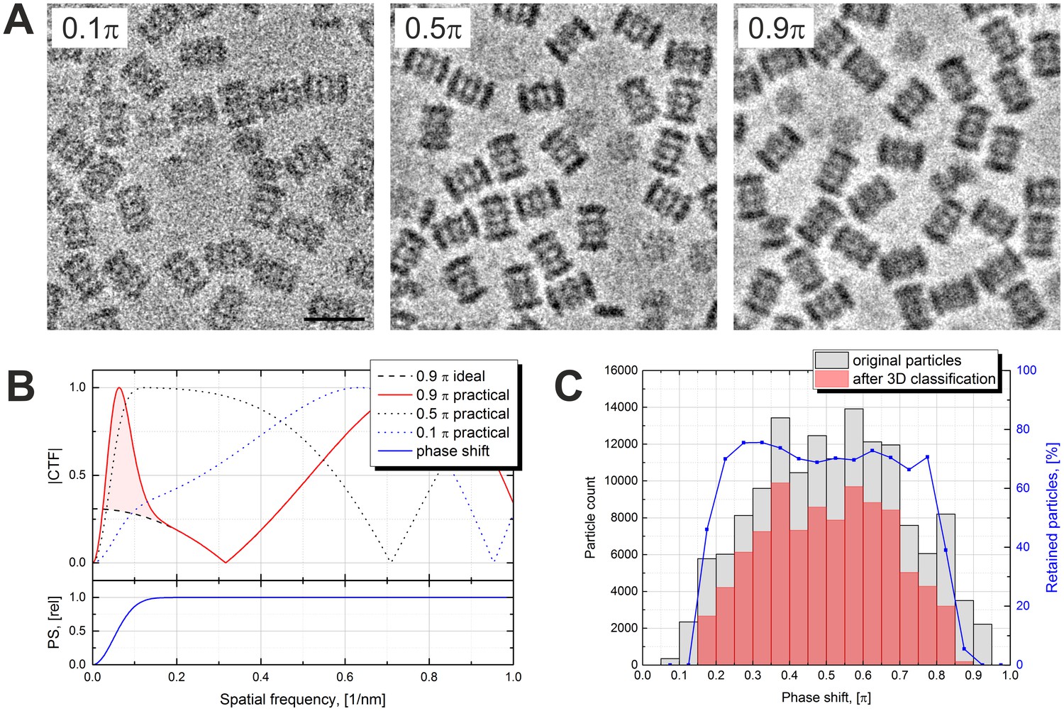
Effects of the Volta phase plate phase shift on the image appearance and the contrast transfer function.
(A) Examples of images at low (0.1 π), optimal (0.5 π) and high (0.9 π) phase shifts. (B) Simulated contrast transfer functions (CTF) at 500 nm defocus and different phase shifts (top). Relative phase shift (PS) profile of the Volta phase plate (bottom). The black dashed line represents a CTF of an ideal (delta function) phase plate with 0.9 π phase shift. (C) Phase shift histograms before (gray) and after (red) 3D classification of the particles. Particles with low (<0.2 π) and high (>0.8 π) phase shifts were predominantly rejected. The blue line (right vertical axis) is the particle retention (after vs before 3D classification). Scale bar: 20 nm.
Figure 3
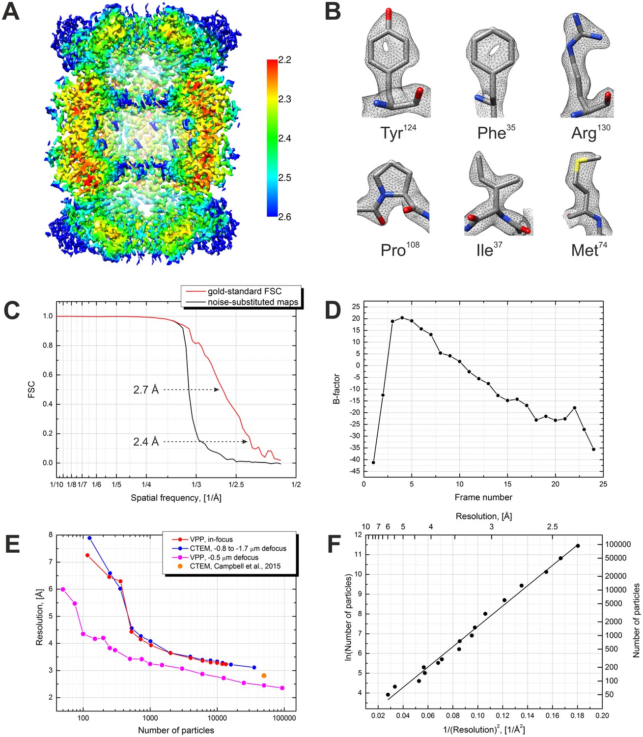
Results from the 3D reconstruction of the 20S proteasome dataset with Relion particle polishing.
(A) Cross-section of the 3D map colored according to the local resolution. (B) Examples of sidechain details. (C) Fourier shell correlation (FSC) plots indicating a resolution of 2.4 Å according to the gold-standard FSC = 0.143 criterion. (D) Per-frame B-factors calculated during the particle polishing. (E) Resolution as a function of the number of particles measured using random particle subsets. Also shown is a data point from Campbell et al. (2015). (F) Same data as in (E) but with logarithmic and squared reciprocal axes. The slope of the linear fit indicates an overall B-factor of 103 Å2.
Download links
A two-part list of links to download the article, or parts of the article, in various formats.
Downloads (link to download the article as PDF)
Open citations (links to open the citations from this article in various online reference manager services)
Cite this article (links to download the citations from this article in formats compatible with various reference manager tools)
Using the Volta phase plate with defocus for cryo-EM single particle analysis
eLife 6:e23006.
https://doi.org/10.7554/eLife.23006


