Dynamic modulation of decision biases by brainstem arousal systems
- University Medical Center Hamburg-Eppendorf, Germany
- University of Amsterdam, The Netherlands
- Max Planck Institute for Human Development, Germany
- Vrije Universiteit Amsterdam, The Netherlands
- Institute of Psychology, Leiden University, The Netherlands
Figures
Figure 1 with 1 supplement
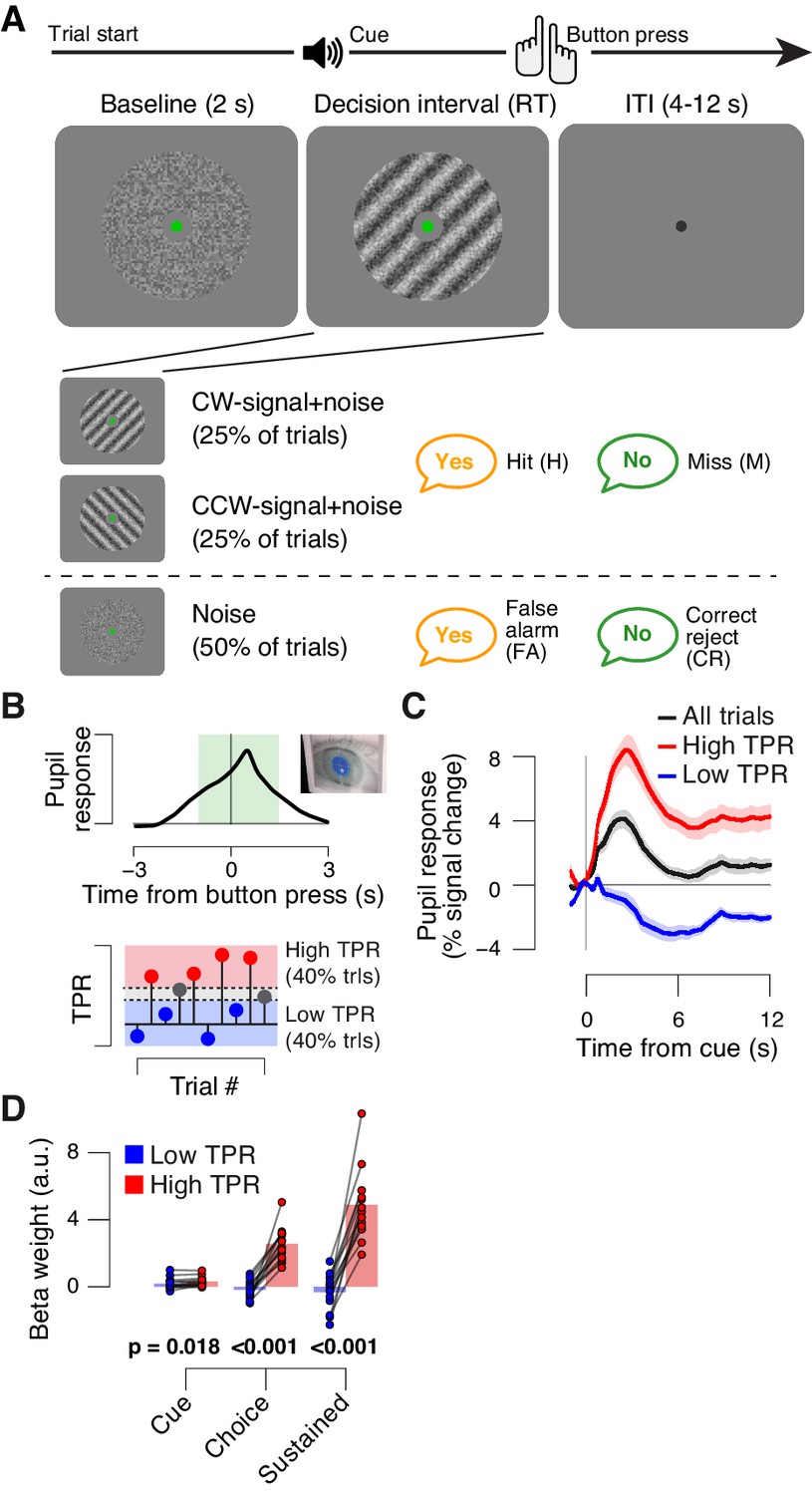
Behavioral task and task-evoked pupil responses.
(A) Yes-no contrast detection task. Top: schematic sequence of events during a signal+noise trial. Subjects reported the presence or absence of a faint grating signal superimposed onto dynamic noise. Bottom left: the signal, if present, was oriented clockwise or counter clockwise on different blocks (known to the subject beforehand). Signal contrast is high for illustration only. Bottom right: trial types. (B) Quantifying task-evoked pupillary response (TPR) amplitude. Top: mean TPR time course of an example subject. Green box, interval for averaging TPR values on single trials. Bottom: trials were pooled into three bins of TPR amplitudes (lowest/highest 40% and intermediate 20%). (C) TPR time course for the three bins. (D) Mean beta weights of transient (cue, choice) and sustained input components under low vs. high TPR, estimated with a general linear model (see Materials and methods; Figure 1—figure supplement 1A,B), separately for low and high TPR trials. Panels C, D: group average (N = 14); shading, s.e.m.; data points, individual subjects; stats, permutation test.
Figure 1—figure supplement 1
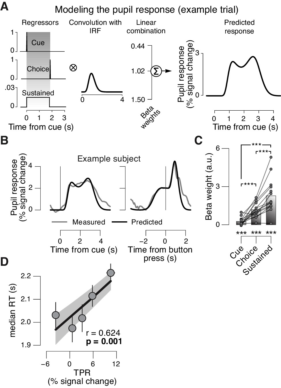
Linear modeling of TPR.
The peripheral system (i.e., nerves and the muscles of the iris [McDougal and Gamlin, 2008]) that transforms central neural inputs originating from the brainstem into TPR is sluggish and acts as a low-pass filter (Hoeks and Levelt, 1993; Korn and Bach, 2016). (A) Linear modeling of TPR (see Materials and methods). We used a previously established general linear model (GLM) to estimate the relative contribution of three putative underlying neural input components (see Materials and methods; [de Gee et al., 2014]). Gray-shaded interval, decision interval (between cue, i.e., decision onset, and button press). The three beta weights are the best fitting parameter estimates for the subject from panel B. IRF, impulse response function. (B) TPR time course from example subject, aligned to cue (left) and button press (right). Gray line, mean TPR (n = 624 trials). Black line, model prediction. The model provided a good fit of the shape of the TPR time course in most subjects. (C) Mean beta weights for all temporal components. As observed previously (de Gee et al., 2014), the predominant input (i.e., largest beta-weight) was a sustained component that spanned the interval between cue- and choice-components. Data points, individual subjects; ***p<0.001. (D) Correlation between TPR and reaction time (RT) (5 bins). Shading or error bars, s.e.m. All panels: Group average (N = 14); stats, permutation test.
Figure 2 with 1 supplement
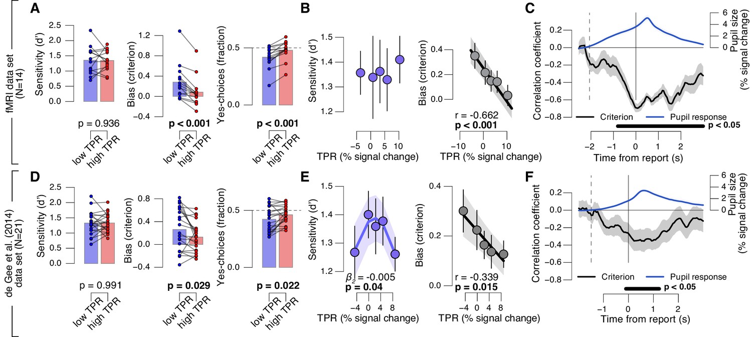
Phasic arousal predicts reduction of choice bias.
(A) Perceptual sensitivity SDT d’ (left), decision bias, measured as SDT criterion (middle) or fraction of ‘yes’-choices (right), for low and high TPR. For the fraction of ‘yes’-choices analysis, we ensured that each TPR bin consisted of an equal number of signal+noise and noise trials (see Materials and methods). Data points, individual subjects. (B) Relationship between TPR and d’ or criterion (5 bins). Linear fits are plotted wherever the first-order fit was superior to the constant fit (see Materials and methods). Quadratic fits are plotted wherever the second-order fit was superior to first-order fit. (C) Sliding window linear correlation between TPR and SDT criterion (5 bins), aligned to button press. Dashed line, median decision onset (cue). The group average pupil response time course is plotted for reference in blue. (D–F) As panels A-C, for an independent data set (de Gee et al., 2014). All panels: group average (N = 14 and N = 21); shading or error bars, s.e.m.; stats, permutation test.
-
Figure 2—source data 3
Table with variable identifiers used in Figure 2—source data 1 and 2.
- https://doi.org/10.7554/eLife.23232.006
-
Figure 2—source data 1
This csv table contains the data for Figure 2 panel A.
- https://doi.org/10.7554/eLife.23232.007
-
Figure 2—source data 2
This csv table contains the data for Figure 2 panel D.
- https://doi.org/10.7554/eLife.23232.008
Figure 2—figure supplement 1
Phasic arousal predicts reduction of choice bias.
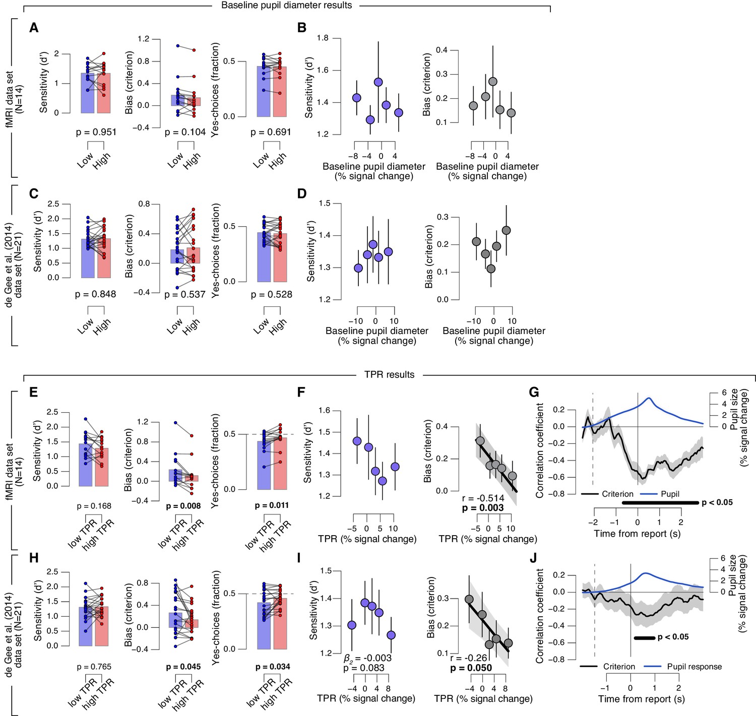
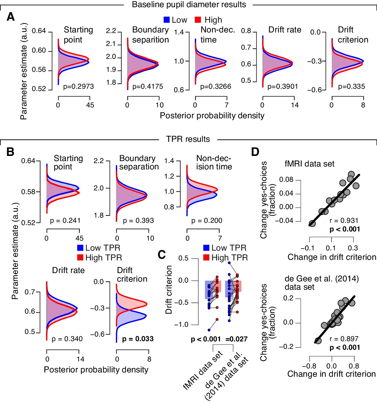
(A–D) As main Figure 2 panels A, B, D, E, but now after splitting trials by (or as a function of) baseline pupil diameter, quantified as the mean pupil size in the 0.5 s before decision interval onset. (E–J) As main Figure 2 panels A-F, but now without removing trial-to-trial variations from TPR due to reaction time (RT). The pattern of results is qualitatively identical to the one in Figure 2. All panels: group average (N = 14); shading or error bars, s.e.m.; stats, permutation test. Panels A, C, E, H: data points, individual subjects.
Figure 3
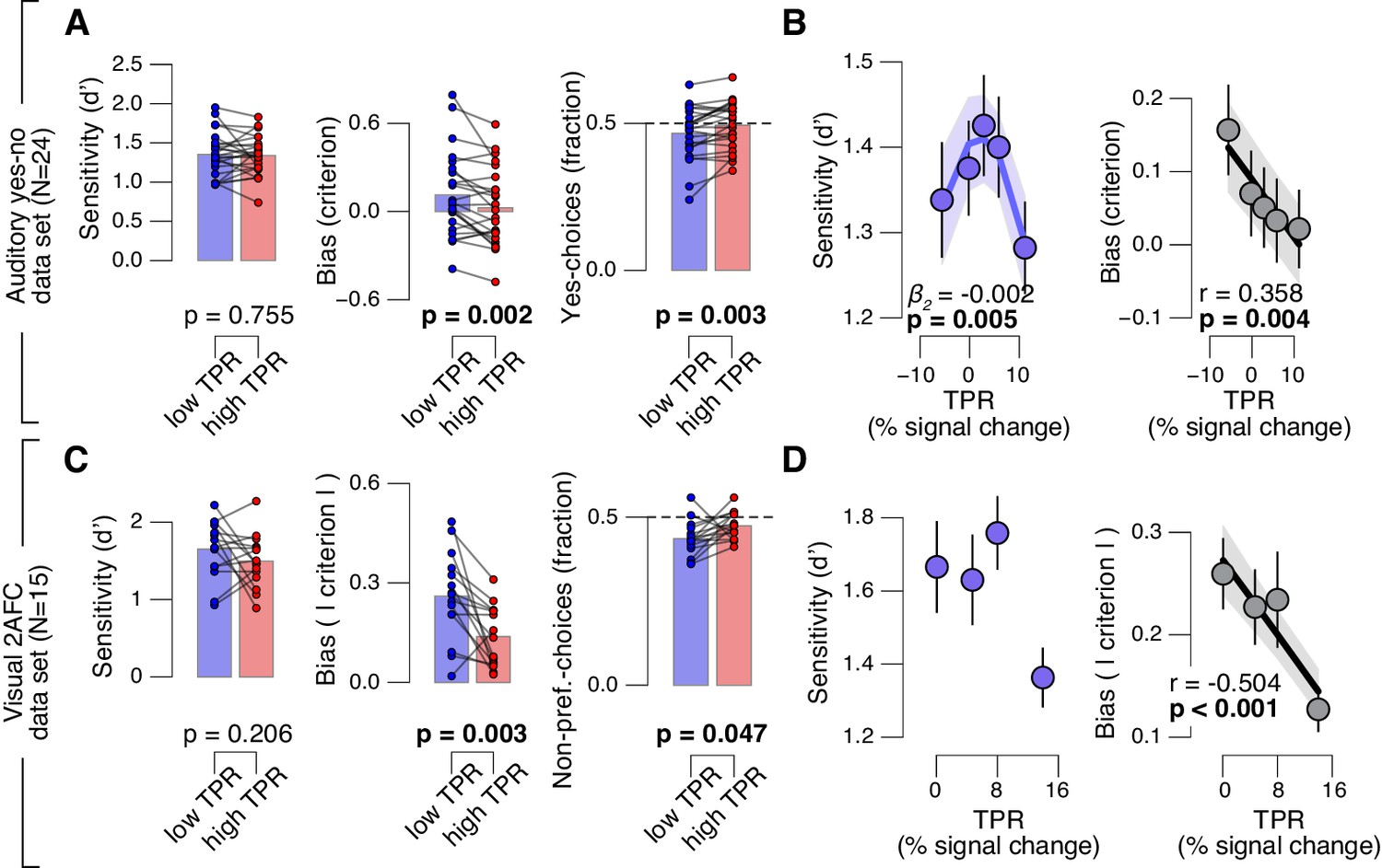
Arousal-linked bias reduction generalizes to other choice tasks.
(A) Perceptual sensitivity (d’; left) and decision bias, measured as criterion (middle) or fraction of ‘yes’-choices (computed as for Figure 2A, right), for low and high TPR. Data points, individual subjects. (B) Relationship between TPR and d’ or criterion (5 bins). Linear fits were plotted wherever the first-order fit was superior to the constant fit (see Materials and methods). Quadratic fits were plotted wherever the second-order fit was superior to first-order fit. (C) Perceptual sensitivity (d’, left) and decision bias, measured as absolute criterion (middle) or fraction of non-preferred choices (right), for low and high TPR. For the fraction of non-preferred choices analysis, we ensured that each TPR bin consisted of an equal number of motion up and down trials (see Materials and methods). (D) Relationship between TPR and d’ or absolute criterion (4 bins instead of 5, because of fewer trials per subject, see Materials and methods). All panels: group average (N = 24 and N = 15); shading or error bars, s.e.m.; stats, permutation test.
-
Figure 3—source data 3
Table with variable identifiers used in Figure 3—source data 1 and 2.
- https://doi.org/10.7554/eLife.23232.011
-
Figure 3—source data 1
This csv table contains the data for Figure 3 panel A.
- https://doi.org/10.7554/eLife.23232.012
-
Figure 3—source data 2
This csv table contains the data for Figure 3 panel C.
- https://doi.org/10.7554/eLife.23232.013
Figure 4 with 2 supplements
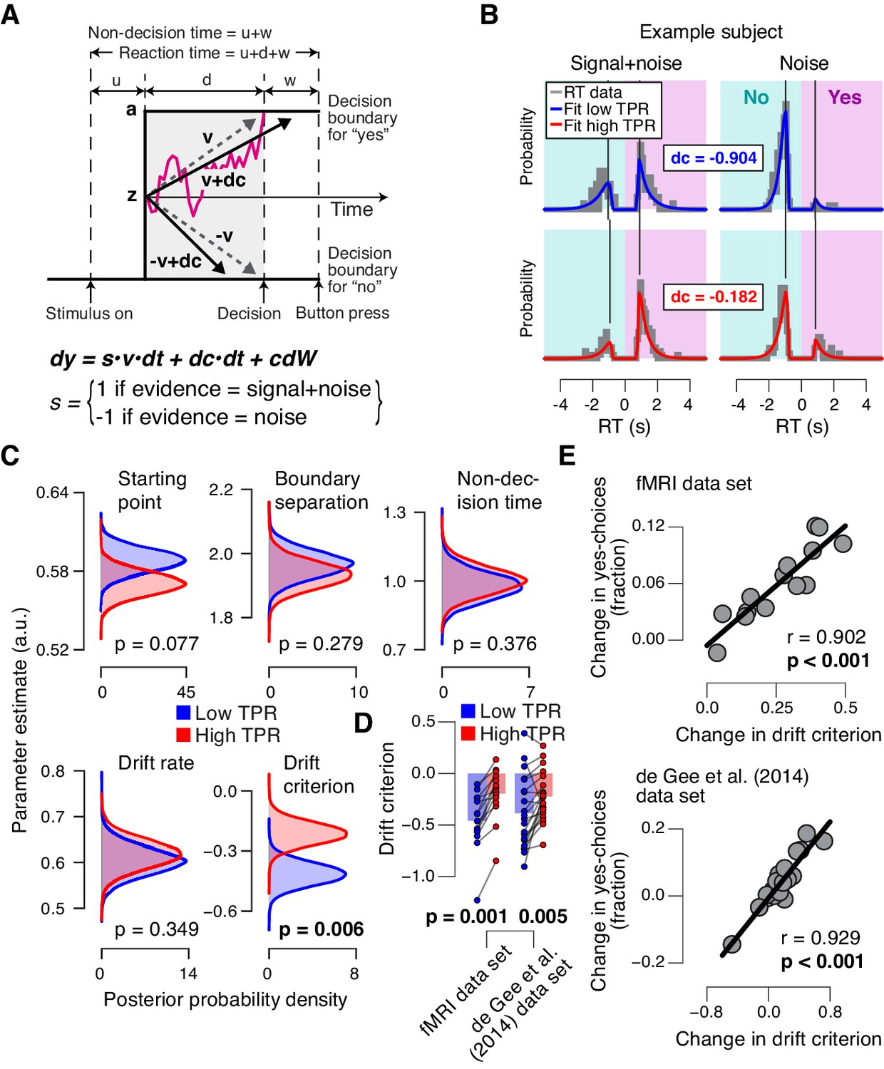
Phasic arousal predicts reduction of accumulation bias.
(A) Schematic and simplified equation of drift diffusion model accounting for RT distributions for ‘yes’- and ‘no’-choices (‘stimulus coding’; see Materials and methods). Notation: dy, change in decision variable y per unit time dt; v•dt, mean drift (multiplied with 1 for signal+noise trials, and −1 for noise trials); dc•dt, drift criterion (an evidence-independent constant added to the drift); and cdW, Gaussian white noise (mean = 0, variance = c2 dt). (B) RT distributions of one example subject for ‘yes’- and ‘no’-choices, separately for signal+noise and noise trials and separately for low and high TPR. RTs for ‘no’-choices were sign-flipped for illustration purposes. Straight lines, mode (i.e., maximum) of the fitted RT distributions. Please note that TPR predicts an increased fraction of ‘yes’-choices with only a minor change of the mode of the RT distribution, consistent with a drift criterion effect rather than a starting point effect (Figure 4—figure supplement 1). (C) Group-level posterior probability densities for means of parameters. To maximize the robustness of parameter estimates (Wiecki et al., 2013), two data sets were fit jointly (the current fMRI and our previous study (de Gee et al., 2014); N = 35). Starting point (z) is expressed as a proportion of the boundary separation (a). (D) Drift criterion point estimates for low and high TPR trials, separately for both data sets (N = 14 and N = 21, respectively). Data points, individual subjects; stats, permutation test. (E) Change in fraction of ‘yes’-choices for low vs. high TPR trials, plotted against change in drift criterion. Data points, individual subjects.
-
Figure 4—source data 2
Table with variable identifiers used in Figure 4—source data 1.
- https://doi.org/10.7554/eLife.23232.015
-
Figure 4—source data 1
This csv table contains the data for Figure 4 panel D.
- https://doi.org/10.7554/eLife.23232.016
Figure 4—figure supplement 1
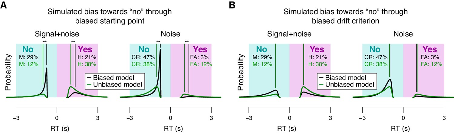
Effects of starting point vs. drift criterion on RT distributions.
Analytical RT distributions sorted by the four SDT categories: ‘yes’- and ‘no’-choices, as well as signal+noise and noise trials. Within each category, RT distributions are shown separately for a biased model (black) and an unbiased model (green), whereby biased model refers to a model producing unequal fractions of ‘yes’- and ‘no’-choices. RTs for ‘no’-choices were sign-flipped for illustration purposes. A conservative choice bias was implemented in two separate mechanisms in the two panels, both producing the same change on the fraction of choices. These mechanisms have distinguishable effect on the shape of the RT distributions, most evident in the mode. (A) Conservative choice bias through setting the starting point of the accumulation process closer to the ‘no’-bound. Straight lines, mode (i.e., maximum) of the analytical RT distributions. A shift in starting point produced a substantial shift of the mode of the RT distribution (compare black and green vertical lines). (B) Conservative choice bias through changing drift criterion in the direction of the ‘no’-bound. This shift in drift criterion had a negligible effect on the mode of RT distributions (green and black vertical lines are on top of one another).
Figure 4—figure supplement 2
Phasic arousal predicts reduction of accumulation bias.
(A) As main Figure 4C, but now after splitting trials by baseline pupil diameter, quantified as the mean pupil size in the 0.5 s before decision interval onset. (B–D) As main Figure 4C–E, but now without removing trial-to-trial variations from TPR due to reaction time (RT). The pattern of results is qualitatively identical. Data points, individual subjects; stats, permutation test.
Figure 5 with 1 supplement
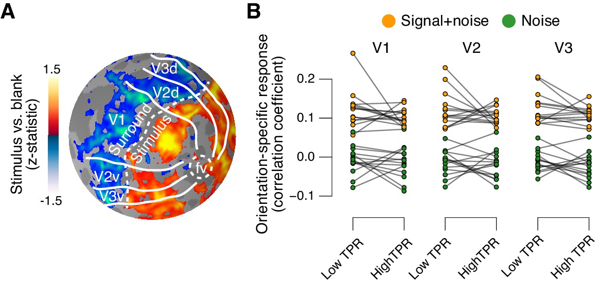
Phasic arousal does not boost sensory responses in visual cortex.
(A) Map of fMRI responses during stimulus localizer runs (see Materials and methods); example subject. V1-V3 borders were defined based on a separate retinotopic mapping session. ‘Stimulus sub-regions’, regions with positive stimulus-evoked response; ‘surround sub-regions’, regions with negative stimulus-evoked response. (B) Orientation-specific fMRI responses in ‘center’ sub-regions of V1-V3, separately for signal+noise and noise trials, and separately for low and high TPR trials. Statistical tests are reported in main text. Data points, individual subjects (N = 14); stats in main text.
Figure 5—figure supplement 1
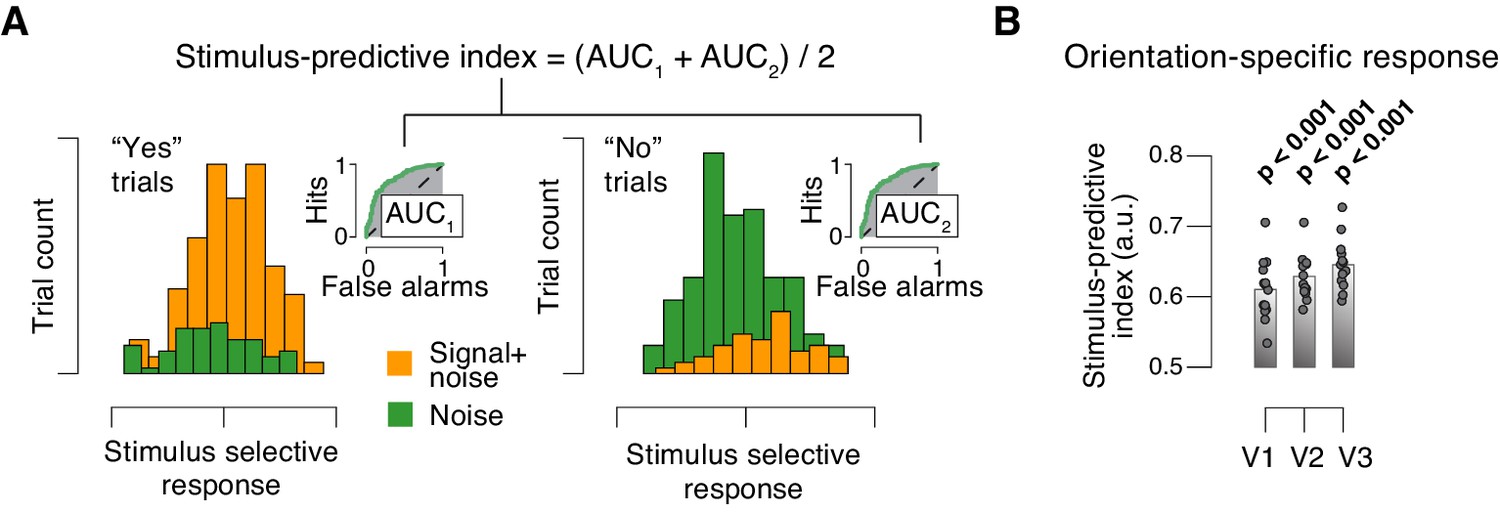
Quantifying single-trial reliability of stimulus-specific responses.
(A) The stimulus-predictive index was calculated from the receiver operating characteristic (ROC) curve, separately for ‘yes’- (left) and ‘no’-choices (right). Each panel shows distributions (taken from area V1 of one example subject) of single-trial pattern responses (see Materials and methods) for signal+noise and noise conditions. ROC curves (insets) were constructed by shifting a criterion across both distributions, and plotting against one another, for each position of the criterion, the fraction of trials for which responses were larger than the criterion. The area under the resulting ROC curve (AUC; grey shading), here referred to as ‘predictive index’, quantifies the probability with which an ideal observer can predict the signal presence from the single-trial fMRI response. Predictive indices calculated separately for ‘yes’- and ‘no’-trials were pooled (averaged) into a single stimulus-predictive index. The predictive index in this example was 0.63. (B) Stimulus-predictive indexes for orientation-specific responses (signal+noise vs. noise, irrespective of choice; see Materials and methods and panel A). Data points, individual subjects; stats, permutation test.
Figure 6
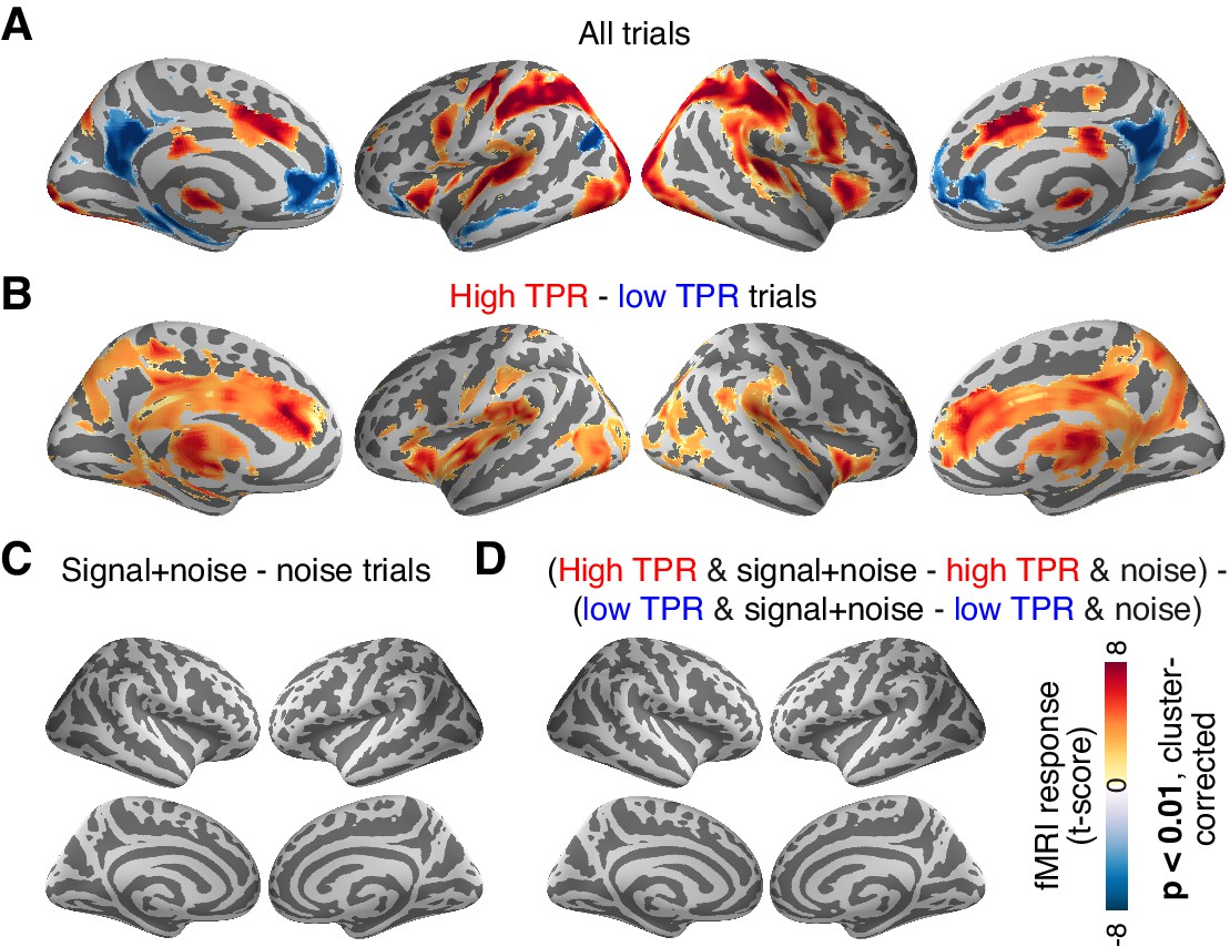
Cortex-wide fMRI correlates of phasic arousal and stimulus.
(A) Functional map of task-evoked fMRI responses computed as the mean across all trials. (B) As panel A, but for the contrast high vs. low TPR trials. (C) As panel A, but for the contrast signal+noise vs. noise. (D) As panel A, but for the interaction between TPR (2 levels) and stimulus (2 levels). All panels: functional maps are expressed as t-scores computed at the group level (N = 14) and presented with cluster-corrected statistical threshold (see Materials and methods).
Figure 7 with 1 supplement
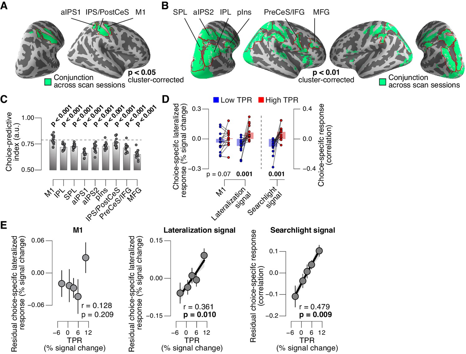
Phasic arousal predicts change of cortical decision signals.
(A) Conjunction of session-wise maps of logistic regression coefficients of choice against fMRI lateralization (see Figure 7—figure supplement 1A for individual sessions). Tested against 0.5 at group level; red outlines, ROIs used for further analyses. (B) Conjunction of session-wise maps of searchlight choice classification precision scores (see Figure 7—figure supplement 1C for individual sessions). Tested against 0.5 at group level; red outlines, ROIs used for further analyses. (C) Choice-predictive indexes for choice-specific responses (‘yes’ vs. ‘no’, irrespective of stimulus; see Materials and methods and Figure 7—figure supplement 1G). Dashed line, index for M1, which can be regarded as a reference given the measurement noise. Data points, individual subjects. (D) Choice-specific responses, obtained through mapping lateralization (M1 and the combined ‘lateralization signal’, i.e., regions from Figure 7A excluding M1; see Materials and methods) and through searchlight classification (combined ‘searchlight signal’, i.e., all regions from Figure 7B), for low and high TPR trials. Data points, individual subjects. (E) Correlation between TPR and M1 (left), or the combined ‘lateralization signal’ (middle), or the combined ‘searchlight signal’ (right) (5 bins). In all cases, the effect of the physical stimulus was removed (see Materials and methods). Shading or error bars, s.e.m. All panels: group average (N = 14); stats, permutation test.
Figure 7—figure supplement 1
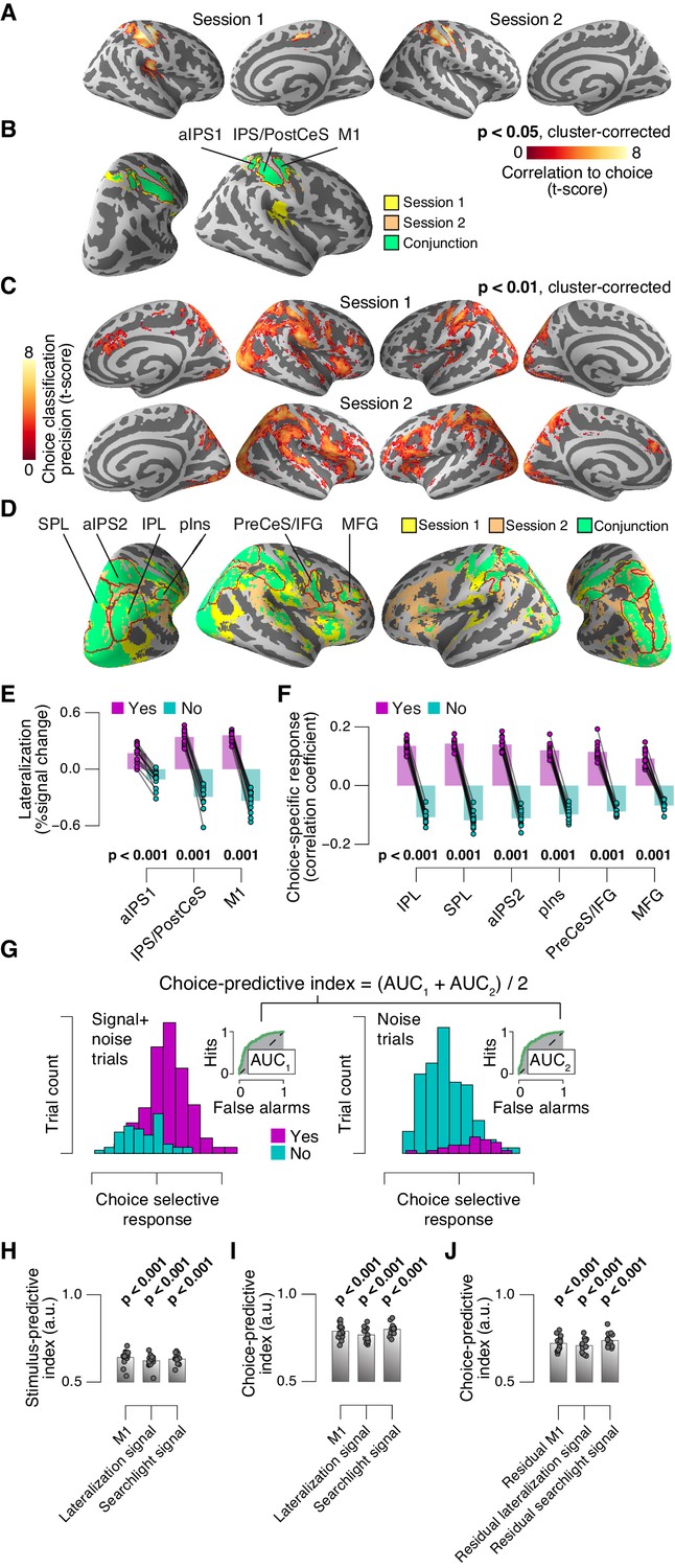
Identifying choice-specific cortical signals.
(A) Session-wise maps map of logistic regression coefficients (choice against fMRI lateralization). (B) Overlay of both maps from panel A, to identify robust and replicable choice-specific responses. (C) Session-wise maps of searchlight choice classification precision scores. (D) Overlay of both maps from panel C, to identify robust and replicable choice-specific responses. A-D: all tested against 0.5 at group level; red outlines, ROIs used for further analyses. (E,F) Choice-specific responses in ROIs from panels B and D, respectively, separately for ‘yes’- and ‘no’-choices. (G) Quantifying the reliability of choice-specific cortical responses, using single-trial, lateralized M1-responses of an example subject. As Figure 5—figure supplement 1A, but now for prediction of choice, rather than of signal presence. To remove effects of signal presence, we averaged ROC indexes for choice computed separately for signal+noise and noise conditions. The resulting measure is analogous to ‘choice probability’ employed in monkey electrophysiology. The predictive index in this example was 0.82. All panels: group average (N = 14); data points, individual subjects; stats, permutation test. aIPS, anterior intraparietal sulcus; IPS, intraparietal sulcus; PostCeS, postcentral sulcus; M1, primary sensorimotor cortex (hand area); SPL, superior parietal lobule; IPL, inferior parietal lobule; pINS, posterior insular cortex; PreCeS, precentral sulcus; IFG, inferior frontal gyrus; MFG, medial frontal gyrus. (H) Stimulus-predictive indexes for choice-specific responses (‘yes’ vs. ‘no’, without first taking out effects of stimulus as in panel G). ‘Combined lateralization’ signal, weighted sum of choice-specific responses across ROIs obtained through mapping significant lateralization with respect to the hand movement (except M1; from Figure 7A; see Materials and methods). ‘Combined searchlight’ signal, weighted sum of choice-specific responses across ROIs obtained through searchlight classification (from Figure 7B). (I) As panel H, but for choice-predictive indexes (signal+noise vs. noise, without first taking out effects of choice as in Figure 5—figure supplement 1A). (J) As panel I, but after removing effects of physical stimulus via linear regression (see Materials and methods). All panels: group average (N = 14); data points, individual subjects; ***p<0.001; stats, permutation test.
Figure 8 with 1 supplement
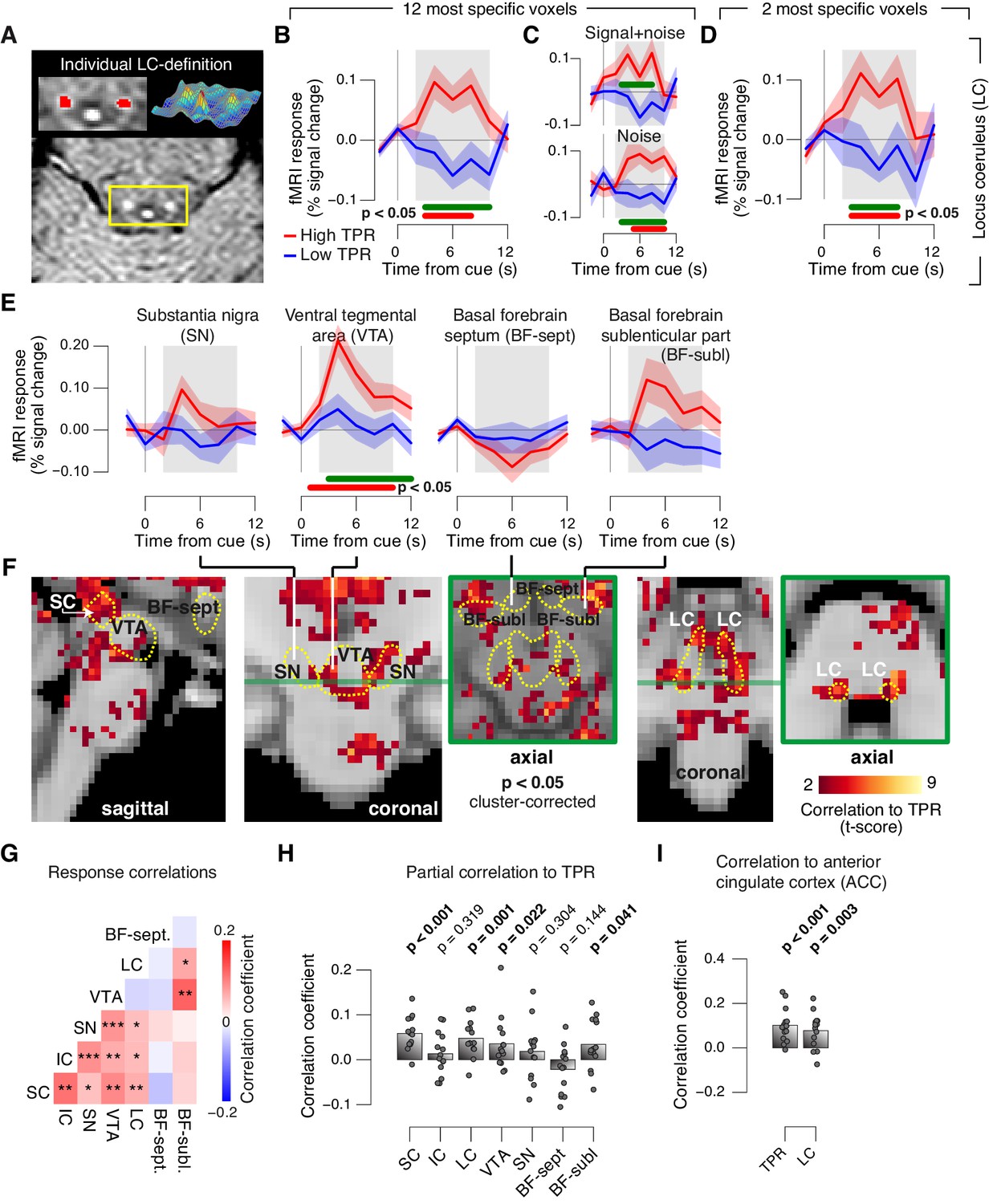
Pupil responses reflect responses of a network of brainstem nuclei.
(A) Delineation of LC by structural scan. The LC corresponds to two hyper-intense spots; example subject (see Figure 8—figure supplement 1 for all subjects). Left inset, magnification of yellow box with LC ROI. Right inset, three-dimensional representation of signal intensity levels in yellow box. (B) Task-evoked LC responses for low and high TPR. Red bar, high TPR time course significantly different from zero; green bar, high TPR time course significantly different from low TPR time course (p<0.05; cluster-corrected). Grey box, time window for computing scalar response amplitudes. (C) As panel B, but split by signal+noise and noise trials. (D) As panel B, but for the 2 voxels with highest probability of containing the LC. (E) As panel B, but for SN, VTA, and two BF-ROIs. (F) Map of single-trial correlation between TPR and evoked fMRI responses (tested against 0 at group level). Yellow outlines, brainstem nuclei from probabilistic atlases. (G) Matrix of correlations between evoked brainstem fMRI responses. Stats corrected with false discovery rate (FDR). (H) Partial correlation of evoked fMRI responses and TPR. For each ROI, responses of all other ROIs were first removed via linear regression. (I) Correlation between fMRI responses in ACC and TPR and LC. All panels: group average (N = 14); shading, s.e.m.; data points, individual subjects; stats, permutation test.
Figure 8—figure supplement 1
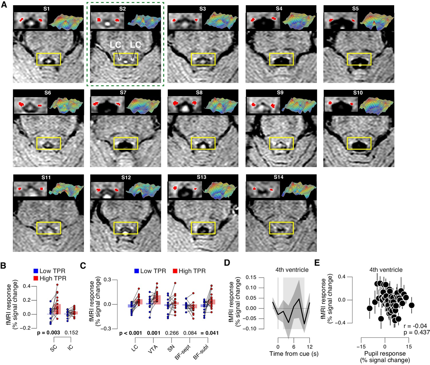
TPR-linked brainstem responses.
(A) As Figure 8A for all subjects. Green outline, subject presented in Figure 8A. (B) Task-evoked responses in SC and IC, separately for low and high TPR trials. (C) As panel B, but for LC, SN, VTA, BF-sept, and BF-subl. Data correspond to Figure 8 panels B and E, but is now represented as bar graphs of task-evoked fMRI response scalar measures (see Materials and methods). (D) Remaining task-evoked fMRI response in the fourth ventricle (after RETROICOR). The fourth ventricle ROI was delineated in the TSE scan, and its response computed by averaging across all voxels covering the ventricle. Gray-shaded interval, task-evoked fMRI response measure time window. Residual signal fluctuations in the fourth ventricle were uncorrelated to task events. Shading, s.e.m. (E) Task-evoked fMRI responses in the fourth ventricle plotted against TPR. Data were binned for display (50 bins). Panels B-E: group average (N = 14). Panels B,C: data points, individual subjects; stats, permutation test.
Figure 9 with 1 supplement
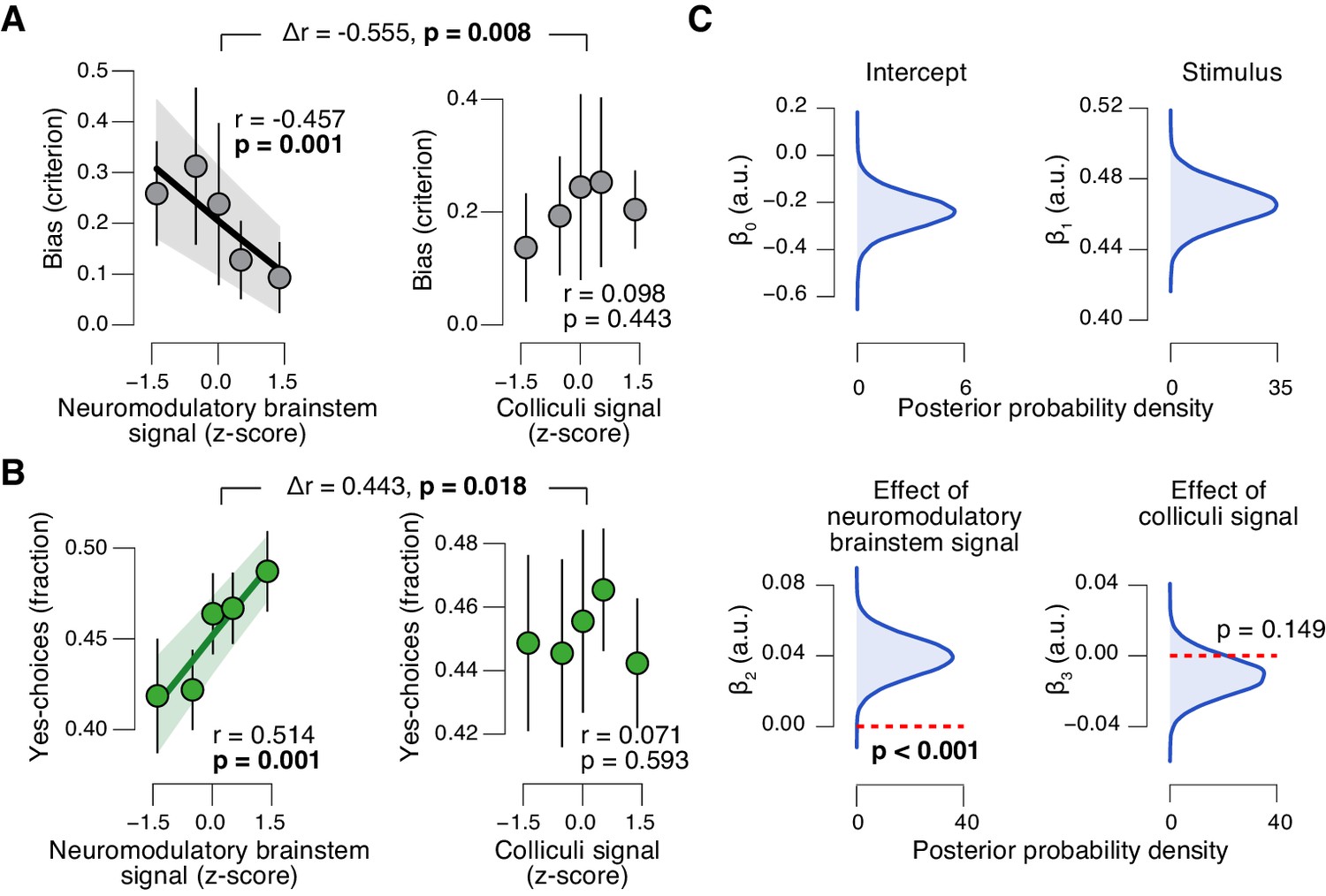
Brainstem neuromodulatory nuclei predict reduction of choice bias.
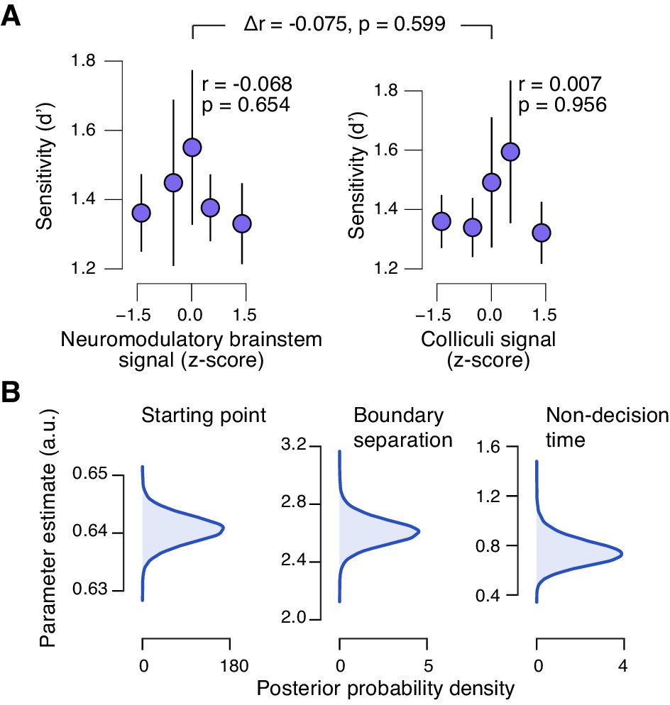
(A) Correlation between decision bias (criterion) and the combined neuromodulatory brainstem signal (linear combination of responses in LC, SN, VTA, BF-sept, and BF-subl maximizing the correlation to TPR; see Materials and methods; left), and the combined colliculi signal (linear combination of responses in SC and IC maximizing the correlation to TPR; right) (5 bins). Stats, permutation test. (B) As panel A but for the correlation to fraction of ‘yes’-choices. (C) Group-level posterior probability densities for means of parameters in the DDM regression model, through which we assessed the trial-by-trial, linear relationship between single-trial drift and the combined neuromodulatory response or the combined colliculi response (see Materials and methods; see Figure 9—figure supplement 1 for the remaining parameters ‘starting point’, ‘boundary separation’ and ‘non-decision time’). All panels: group average (N = 14); shading or error bars, s.e.m.
Figure 9—figure supplement 1
Brainstem responses are not associated to sensitivity.
(A) Correlation between perceptual sensitivity (d’) and the combined neuromodulatory brainstem response (linear combination of responses in LC, SN, VTA, BF-sept, and BF-subl maximizing the correlation to TPR; see Materials and methods), and the combined colliculi response (linear combination of responses in SC and IC maximizing the correlation to TPR) (5 bins). Stats, permutation test. (B) Group-level posterior probability densities for means of the remaining parameters in the DDM regression model, through which we assessed the linear relationship between the trial-by-trial drift and the trial-by-trial combined neuromodulatory response and the combined colliculi response (see Materials and methods). All panels: group average (N = 14); shading or error bars, s.e.m.
Author response image 1
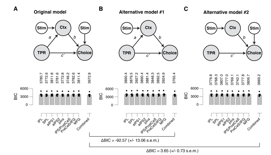
(A) Left: Schematic of original mediation analysis. Ctx, choice-specific cortical response; stim, stimulus (signal+noise vs. noise). All arrows are regressions.Right: BIC values for different choice-specific cortical responses (independently used as the Ctx node). (B) same as panel A, but for alternative model #1 (without stimulus input into Choice). (C) same as panel A, but for alternative model #2 (that does not allow for the indirect path – that is, a model lacking the path from TPR to Ctx).
Author response image 2
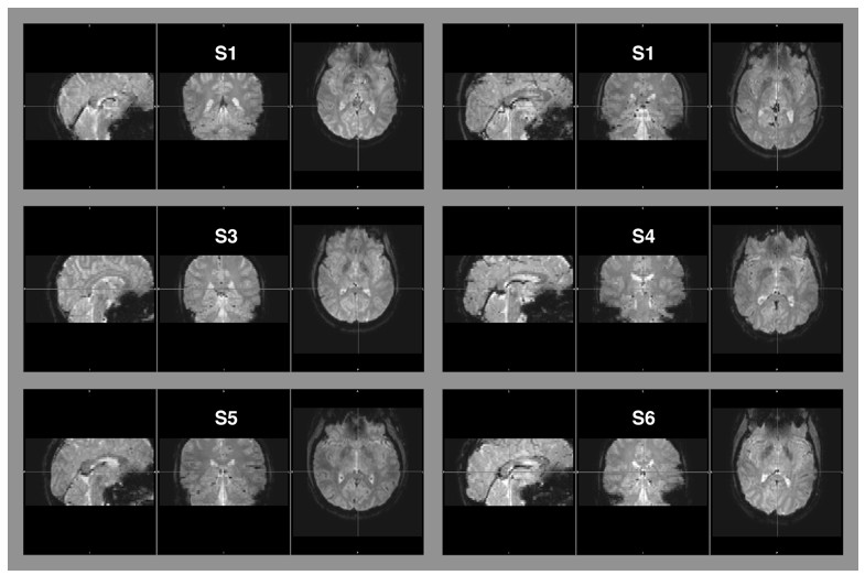
Raw EPI-images of six example subjects.
The images depict the full field of view covered by our measurements. Aliasing artifacts occur when the dimensions of an object exceed the imaging field-of-view, but are within the area covered by the receiver coil. This “wrap-around artifact” is evident as a folding over of surrounding parts into the area of interest, and it is most severe along the phase-encode dimension. In our measurement, the phase-encode dimension was the anterior-posterior axis. No wrap-around artifacts are evident in any of the examples, nor in the other image data that were part of this data set.
Author response image 3
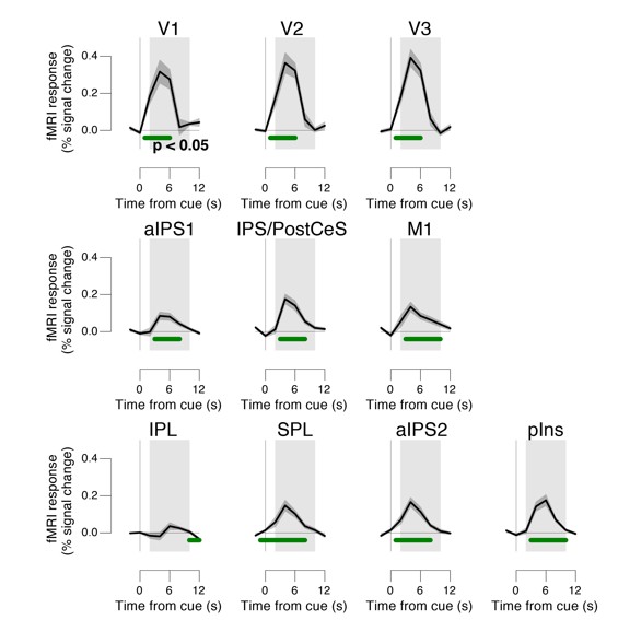
Task-evoked responses across all trials.
Regions of interest were pooled across hemispheres. Green bar, time course significantly different from zero (p < 0.05; cluster-corrected). Grey box, time window for computing scalar response amplitudes.
Download links
A two-part list of links to download the article, or parts of the article, in various formats.
Downloads (link to download the article as PDF)
Open citations (links to open the citations from this article in various online reference manager services)
Cite this article (links to download the citations from this article in formats compatible with various reference manager tools)
Dynamic modulation of decision biases by brainstem arousal systems
eLife 6:e23232.
https://doi.org/10.7554/eLife.23232


