Altered topology of neural circuits in congenital prosopagnosia
- Ben-Gurion University of the Negev, Israel
- Holon Institute of Technology, Israel
- Weizmann Institute of Science, Israel
- Princeton University, United States
- Carnegie Mellon University, United States
Figures
Figure 1
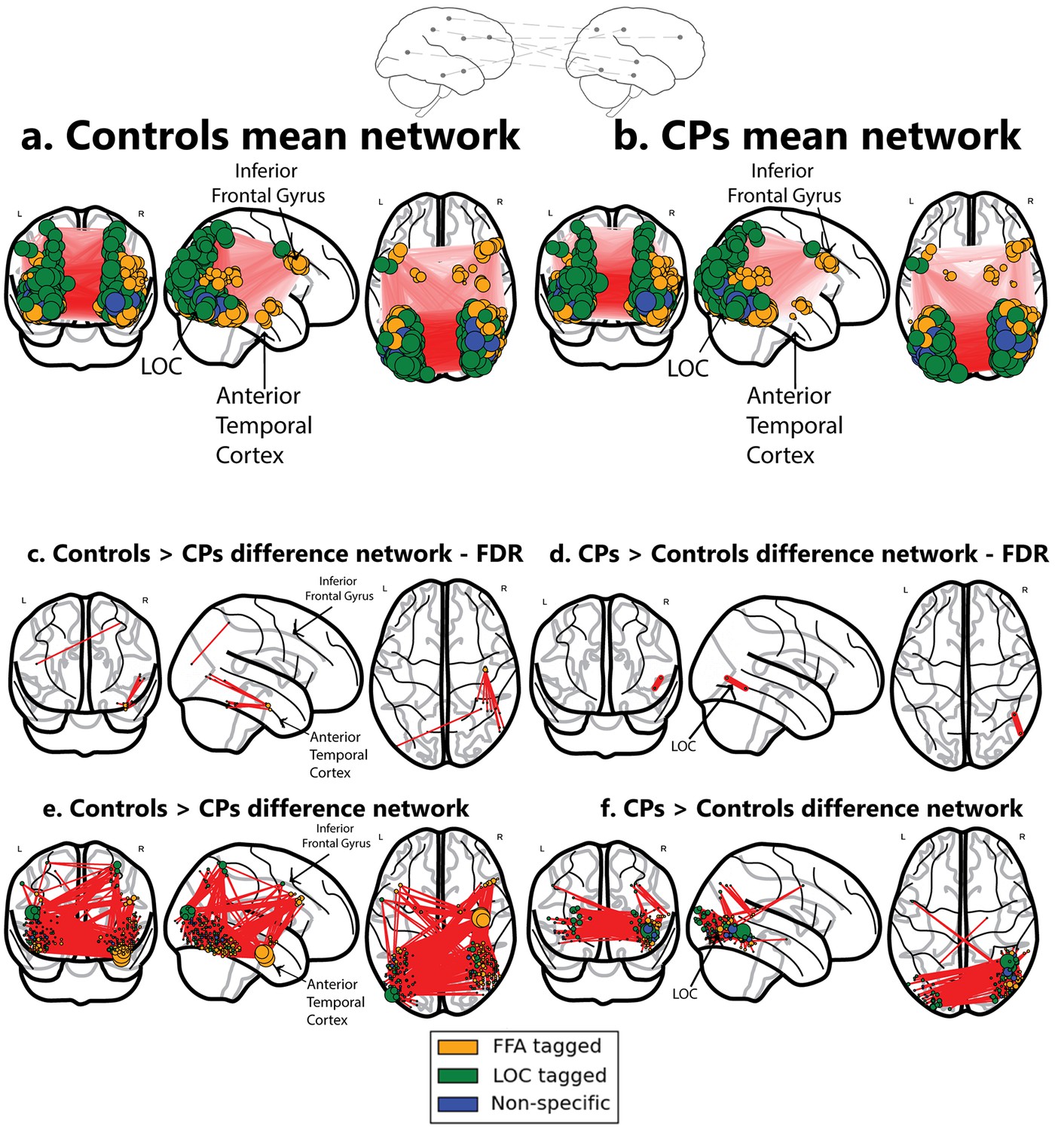
Networks obtained using the ISFC approach.
The top schematic denotes the inter-subject functional correlation approach, which calculates the inter-regional correlations in the brains of different individuals. (a) Mean network obtained from the control group (b) Mean network obtained from the CP group. These mean networks are shown for visualization purposes. For each group, networks are projected on three views of the brain (coronal, sagittal and axial views). The colors of the nodes denote their functional selectivity (face-selective, non-face selective, and nodes which are not exclusively selective for either of these stimuli). For visualization purposes, the size of the node is proportional to its degree (the larger the node, the greater its ISFC). The same conventions are used in all figures. (c) The difference network of controls > CPs after FDR correction (q < 0.05) which reflects the difference between the ISFC values for the controls compared to the CP individuals. The ATL and the inferior frontal gyrus are marked. As is graphically depicted, the ATL serves as the main hub for controls but not for CP. Three nodes, which comprise the ATL, were ranked in the top 10 ranks of degree scores (1-3; see Table 3a). (d) Difference networks obtained from the comparison of CPs > controls. CPs evince a significant difference in ISFC in posterior visual regions. As the FDR correction is very stringent, the differences are also shown for an uncorrected p<0.005 value. Note that this is an arbitrary threshold and was chosen for visualization purposes. (e) For the controls > CPs comparison, ATL serves as the main hub. (f) For the CPs > controls, hyperconnectivity of the network in posterior regions is apparent. For an interactive visualizations of the two networks from controls > CPs and CPs > controls, see https://goo.gl/mCm3OF and https://goo.gl/nctuOb respectively (Dwyer et al., 2015).
Figure 2
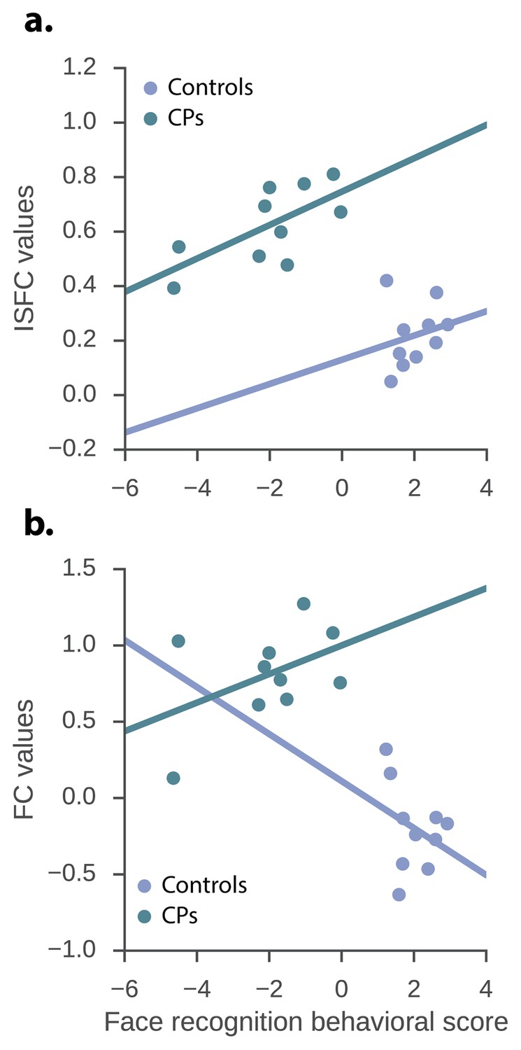
The relation between the neuronal measures and the face recognition behavioral score.
ISFC and FC values of the significant CPs > controls edges and the face recognition behavioral score. (a) ISFC regression – group, as well as ISFC value significantly predict face recognition behavioral score (group: β = −6.08, p<0.0001, t = −6.83, std = 0.87; ISFC value: β = 4.89, p=0.017, t = 2.63, std = 1.85). (b) FC regression - group significantly predict face recognition behavioral score while the FC value does not (group: β = −4.99, p<0.0001, t = −4.68, stde = 1.06; FC value: β = 0.95, p=0.31, t = 1.04, stde = 0.91).
Figure 3
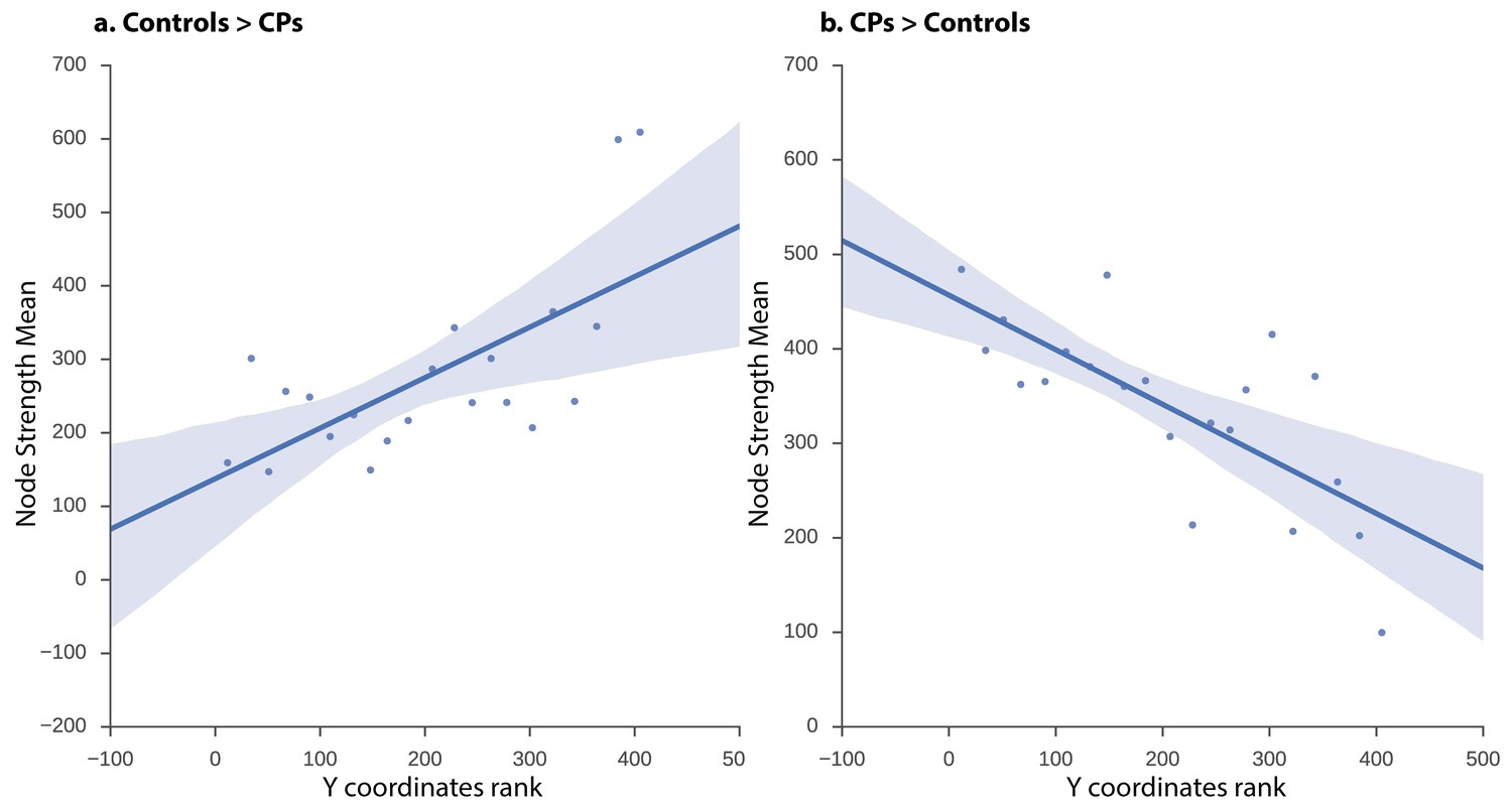
ISFC correlation between strength and node location along posterior-anterior axis.
Linear regression fit with a 95% confidence interval band between the strength measure of the nodes and the Y coordinate ascending rank order of each node binned into 21 equally sized bins for (a) controls > CPs (rs = 0.58, p=0.005) and (b) CPs > controls (rs = −0.70, p=0.0003). The x-axis of the graph denotes the Y coordinates of the 3D MNI space ranked in ascending order, the y-axis of the graph marks the mean strength value of nodes per bin. As is evident, the higher the y-coordinate (more anterior), the higher the strength value for controls > CPs and the lower the value for CPs > controls.
Figure 4
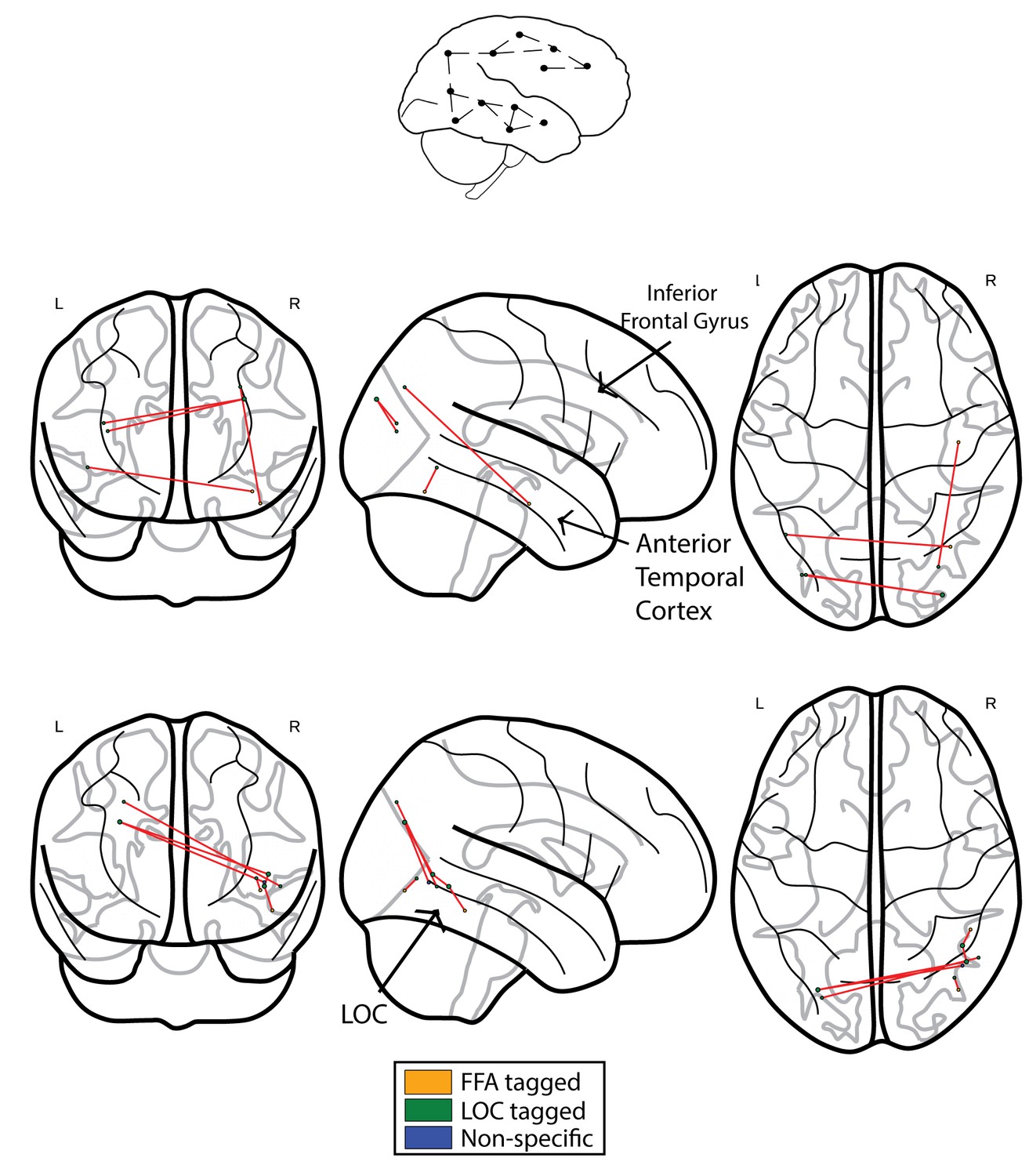
Networks obtained using the FC approach.
The top schematic denotes the intra-subject functional correlation, which calculates the inter-regional correlations within the brains of single individuals. (a) The FC difference network of controls>CPs. This comparison reflects the difference between the FC correlation coefficient values of the controls compared to the group of CP individuals. The maps are presented following the application of the FDR correction (q < 0.05). (b) Difference networks obtained from the comparison of FC in CPs>controls.
Tables
Table 1
CP behavioral scores ordered by severity as indicated by performance on the CFMT.
| Participant | Sex | Age | Famous faces questionnaire | CFMT (total) | ||
|---|---|---|---|---|---|---|
| % corr. | Z- score | |||||
| BL | F | 18 | 20 | -4.88 | 28 | -4.15 |
| BQ | F | 29 | 16 | -4.92 | 30 | -3.89 |
| KG | F | 49 | 75 | -0.69 | 33 | -3.5 |
| ON (Avidan et al., 2014) | F | 48 | 60.7 | -1.77 | 35 | -3.23 |
| MT (Nishimura et al., 2010), (Avidan et al., 2011), (Behrmann and Avidan, 2005), (Thomas et al., 2009), (Avidan and Behrmann, 2008), (Humphreys et al., 2007) , (Behrmann et al., 2007), (Avidan et al., 2014) | M | 50 | 62.5 | -1.64 | 36 | -3.11 |
| WA (Nishimura et al., 2010), (Avidan et al., 2014) | F | 23 | 45.7 | -2.91 | 40 | -2.58 |
| KE (Avidan et al., 2011), (Thomas et al., 2009), (Avidan et al., 2014) | F | 67 | 42.9 | -3.12 | 40 | -2.58 |
| TD (Nishimura et al., 2010), (Avidan et al., 2011), (Avidan et al., 2014) | F | 38 | 46.4 | -2.85 | 41 | -2.45 |
| MN (Nishimura et al., 2010), (Avidan et al., 2014) | F | 50 | 60.7 | -1.77 | 52 | -1 |
| BT (Avidan et al., 2011), (Avidan et al., 2014) | M | 32 | 55.3 | -2.18 | 58 | -0.21 |
| CP Mean ± s.d | 40.4± 15.03 | 48.52 ± 18.72 | 39.3 ± 9.41 | |||
| Control Mean ± s.d | 39.3 ± 13.4 | 91.57±6.24 | 58.28 ± 5.87 | |||
-
The table shows the age and gender of participants and their performance (raw values and z-normalized scores relative to a large control group) on the famous faces questionnaire and CFMT. Note that 7 of the 10 CPs have participated in previous behavioral (3 CPs), and imaging (7 CPs) studies; additional behavioral measures for the CP individuals can be found in these references. Specific details regarding diagnostic and inclusion criteria can be found in the Materials and methods section and in the related studies. The average performance on the famous faces questionnaire and the CFMT of the controls who participated in the present study is also provided (t-test comparing performance across the CP and the controls, for famous faces questionnaire p<0.0005 and CFMT p<0.0005).
Table 2
Coordinates of the ATL nodes, and the calculated values of the within module weighted degree and participation coefficient.
| Number Of Voxels | MNI center coordinates | Within module weighted degree | Participation coefficient |
|---|---|---|---|
| 23 | 42, -14, -26 | 3.91 | 0.58 |
| 13 | 40, -10, -32 | 4.81 | 0.58 |
| 20 | 40, -12, -28 | 5.15 | 0.59 |
| Voxels | 40, -10, -32 | Weighted Mean: | Weighted Mean: |
| Sum: | |||
| 55 | 4.63 | 0.58 |
-
Coordinates of the ATL are in line with (Rajimehr et al., 2009; Pyles et al., 2013). To assess whether the differences are specific to face-selective nodes, the ratio of face-selective nodes and non-face selective nodes connected to the ATL nodes was quantified using within-module weighted degree and participation coefficient. Within-module weighted degree measures the ISFC level of a node within its module. In this analysis, a module is defined as one of the three types of functional tags (faces, non-faces and overlap). Note that this definition is different from the graph theoretical modularity measure as used in the first section of the results. The participation coefficient measures the inter-module diversity of the nodes' connections, meaning how much a node is connected not only within its own module but across modules (Guimerà and Nunes Amaral, 2005).
-
This resulted in a within-module weighted degree weighted average of 4.63 and a participation coefficient weighted average of 0.58. Values greater than 2 are considered as a 'module hub'. Additionally, 'module hubs' with a participation coefficient between 0.3 and 0.75 are treated as 'connector hubs', that is hubs with many connections to most of the other modules (Guimerà and Nunes Amaral, 2005). Importantly, based on these standard values, the differences between controls and CPs, assigned to the ATL, are not a priori face specific.
Table 3
Rank of top 10 nodes obtained from the comparisons of CP and the control group.
| a. Controls>CPs | b. CPs>Controls | ||
|---|---|---|---|
| Rank | Region Name | Rank | Region Name |
| 1,2,3 | Anterior temporal Cortex (faces) | 1,3,4,5,9,10 | Right inferior temporal gyrus (non-faces) |
| 8 | Right Temporal Occipital Fusiform (faces) | 2 | Left lateral occipital cortex (non-faces) |
| 4 | Left TOS (non-faces) | 6 | Right lateral occipital cortex (non-faces) |
| 7 | Left Lateral Occipital cortex (non-faces) | 7 | Right lateral occipital cortex (faces) |
| 9,10 | Left inferior frontal gyrus (faces) | 8 | Right lateral occipital cortex (non-selective) |
| 5,6 | Amygdala left (faces) | ||
-
The 10 nodes with the highest node strength obtained from the Controls>CPs (a) and CPs>Controls (b) difference networks. Anatomical locations, which are based on 'The atlas of the human brain' (Mai et al., 2008) and validated by an expert, are provided for each node. Note that, in the controls>CP network, most of the nodes were face selective, while in the CP>controls network, only a single node was face selective.
Download links
A two-part list of links to download the article, or parts of the article, in various formats.
Downloads (link to download the article as PDF)
Open citations (links to open the citations from this article in various online reference manager services)
Cite this article (links to download the citations from this article in formats compatible with various reference manager tools)
Altered topology of neural circuits in congenital prosopagnosia
eLife 6:e25069.
https://doi.org/10.7554/eLife.25069


