Early tissue damage and microstructural reorganization predict disease severity in experimental epilepsy
- University of Freiburg, Germany
- Karlsruhe Institute of Technology, Germany
Figures
Figure 1 with 2 supplements
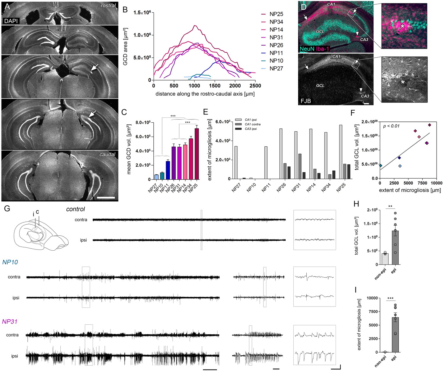
The severity of histological changes associated with HS varies in chronically epileptic mice.
(A) Representative DAPI-stained sections at different levels along the rostro-caudal hippocampal axis showing the extent of GCD (arrow indicates the transition to non-dispersed regions). (B) Corresponding quantitative analysis of the GCD area along the rostro-caudal axis, and (C) the calculated mean GCD volume from all analyzed sections tested for individual kainate-injected mice (one-way ANOVA, Bonferroni’s post-test; ***p<0.001; n = 8). (D) Representative photomicrographs of NeuN (turquoise; neurons) and Iba-1 (magenta; microglia) double immunostaining (upper panel) and Fluoro-Jade B (FJB) staining in consecutive sections. Clusters of amoeboid microglia are tightly associated with FJB-stained dying neurons (arrows and asterisks). (E) Quantitative analysis of cell death-associated microglial scarring in different regions (CA1 ipsi and contra; CA3 ipsi). (F) Regression analysis for the degree of GCD and the extent of microgliosis (summed for all regions) in kainate-injected mice (n = 8; Pearson’s correlation). Kainate-injected mice (NP10, NP11, NP14, NP26, NP27, NP31, NP34) are color-coded. Scale bars in A, 1 mm; in D, 200 µm. (G) Schematic of the mouse brain adapted from Witter and Amaral, 2004. Representative EEG traces of non-epileptic mice (controls or mice displaying only single epileptic spikes, NP10) and one example of an epileptic mouse displaying both epileptic spikes and paroxysmal discharges (NP31). Horizontal scale bars (left) 50 s, (middle) 5 s, (right) 0.5 s; vertical scale bar 2 mV. (H–I) Quantitative analysis of the total GCL volume (summed for all analyzed sections) and extent of microgliosis for epileptic (dark grey) and non-epileptic mice (light grey), respectively. Student’s t-test; **p<0.01, ***p<0.001; nnon-epi = 6, nepi = 7. All values are presented as the mean ± SEM.
Figure 1—figure supplement 1
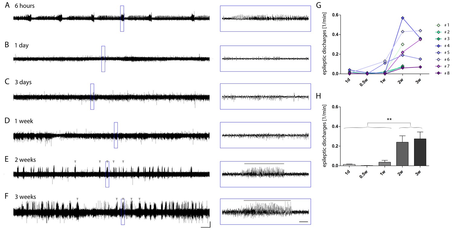
Longitudinal development of epileptiform activity after kainate injection.
(A–F) Representative longitudinal EEG recording of the ipsilateral hippocampus of a kainate-injected mouse. Recordings in the same mouse were repeated at different time points during epileptogenesis (6 hr, 1 day, 3 days, 1 week, 2 weeks and 3 weeks following injection). Detailed images of the respective EEG traces are indicated by blue boxes. Scale bars: Horizontal (left) 200 s and (right) 5 s, vertical 1 mV. Grey arrow heads above the trace and horizontal lines in blue boxes denote examples for high-amplitude recurrent paroxysmal episodes, i.e. epileptic discharges. (G) Quantitative analysis for individual mice (color-coded) and H) for groups. One-way ANOVA, Bonferroni’s post-test, **p<0.01, n1d = 8, n0.5w = 6, n1w = 8, n2w = 8, n3w = 5. Values are presented as the mean ± SEM. Individual recordings were binned for time points: 1 day (recordings on day 1), 0.5 week (rec. on days 3–5), 1 week (rec. on days 6–7), 2 weeks (rec. on days 12–16) and 3 weeks (rec. on days 17–21) after SE.
Figure 1—figure supplement 2

Schematic of the experimental design.
Shown is an overview of the workflow applying multi-modal MRI measurements during the time course of epileptogenesis, video-EEG recording in the chronic stage of the disease and post-hoc IHC. Date was retrospectively correlated to probe the predictive value of putative MRI biomarkers.
Figure 2 with 1 supplement
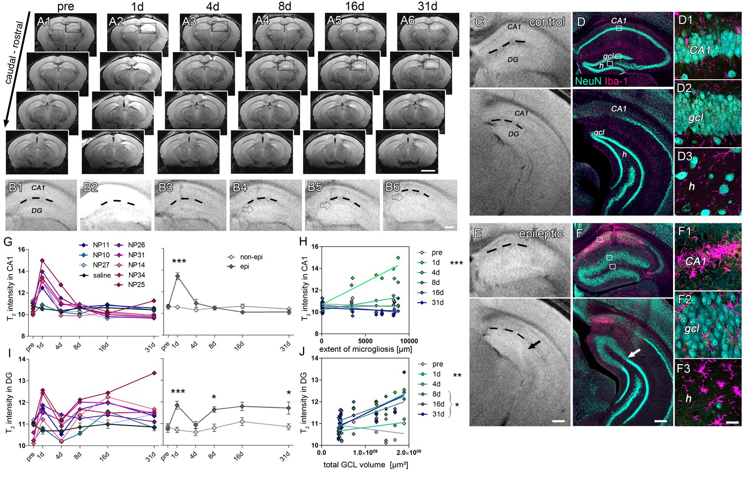
Initial hippocampal damage detected by T2 imaging predicts the degree of HS.
(A1-6) Overview of whole-brain T2 intensity maps along the rostro-caudal axis before (pre) and at distinct time-points following kainate-induced SE (1d, 4d, 8d, 16d and 31d). (B1-6) Enlarged view of the ipsilateral hippocampus. Dashed lines denote the hippocampal fissure. Open arrows mark the GCD. (C–D, E–F) Direct comparison between T2 images and NeuN (turquoise) and Iba-1 (magenta) double-stained sections. Upper and lower panels show the septal and temporal regions of the hippocampus, respectively. Arrows indicate the transition from the dispersed to the non-dispersed GCL. (D1-3, F1-3) High-magnification confocal images corresponding to photomicrographs in D and F display the loss of neurons and accompanied microglial scarring in the CA1 region and the hilus. Principal neurons in the GCL remain intact but are highly dispersed. H, hilus; gcl, granule cell layer. Scale bars: A, 2 mm; B,E,F, 200 µm; F3, 20 µm. (G, I) Quantitative analysis of T2 changes in CA1 and the DG during epileptogenesis plotted for individual animals (left panel: controls, black, n = 5; kainate-injected mice, color-coded), and (right panel) statistically tested for the epileptic (dark grey) and non-epileptic group (light grey). Source data is provided in ‘Figure 2—source data 1'. Two-way ANOVA; Bonferroni’s post-test; *p<0.05, ***p<0.001, nnon-epi = 6, nepi = 7. Values are presented as the mean ± SEM. (H, J) Corresponding linear regression analysis of T2 intensity at distinct time points during epileptogenesis (color-coded) with region-specific histopathological changes in epileptic and non-epileptic mice (n = 13; Pearson’s correlation; corrected for multiple testing; *p<0.05, **p<0.01, ***p<0.001).
-
Figure 2—source data 1
Summary of T2 metrics.
Quantitative values of T2 measurements are listed for individual mice (saline-injected: N12, NP13, NP17, NP28, NP29; kainate-injected: NP10, NP11, NP14, NP25, NP26, NP27, NP31, NP34) and longitudinal time points (pre, 1d, 4d, 8d, 16d, 31d following injection).
- https://doi.org/10.7554/eLife.25742.007
Figure 2—figure supplement 1

T2 changes in the piriform cortex and the amygdala during epileptogenesis.
(A1–3) Representative T2-weighted images of coronal sections prior to kainate injection and at 1 day and 31 days after SE. Enlarged images show the piriform cortex (PirC) and the amygdala (Amyg). Scale bar: 50 µm. (B–C) Quantitative analysis of T2 signal intensity in the piriform cortex and the amygdala, respectively. Values are plotted for individual mice (left panel; controls, black, n = 5; kainate-injected animals color-coded) and for groups (right panel; epileptic, dark grey; non-epileptic, light grey) during epileptogenesis. Two-way ANOVA, Bonferroni’s post-test, nnon-epi = 6, nepi = 7. Values are presented as the mean ± SEM.
Figure 3
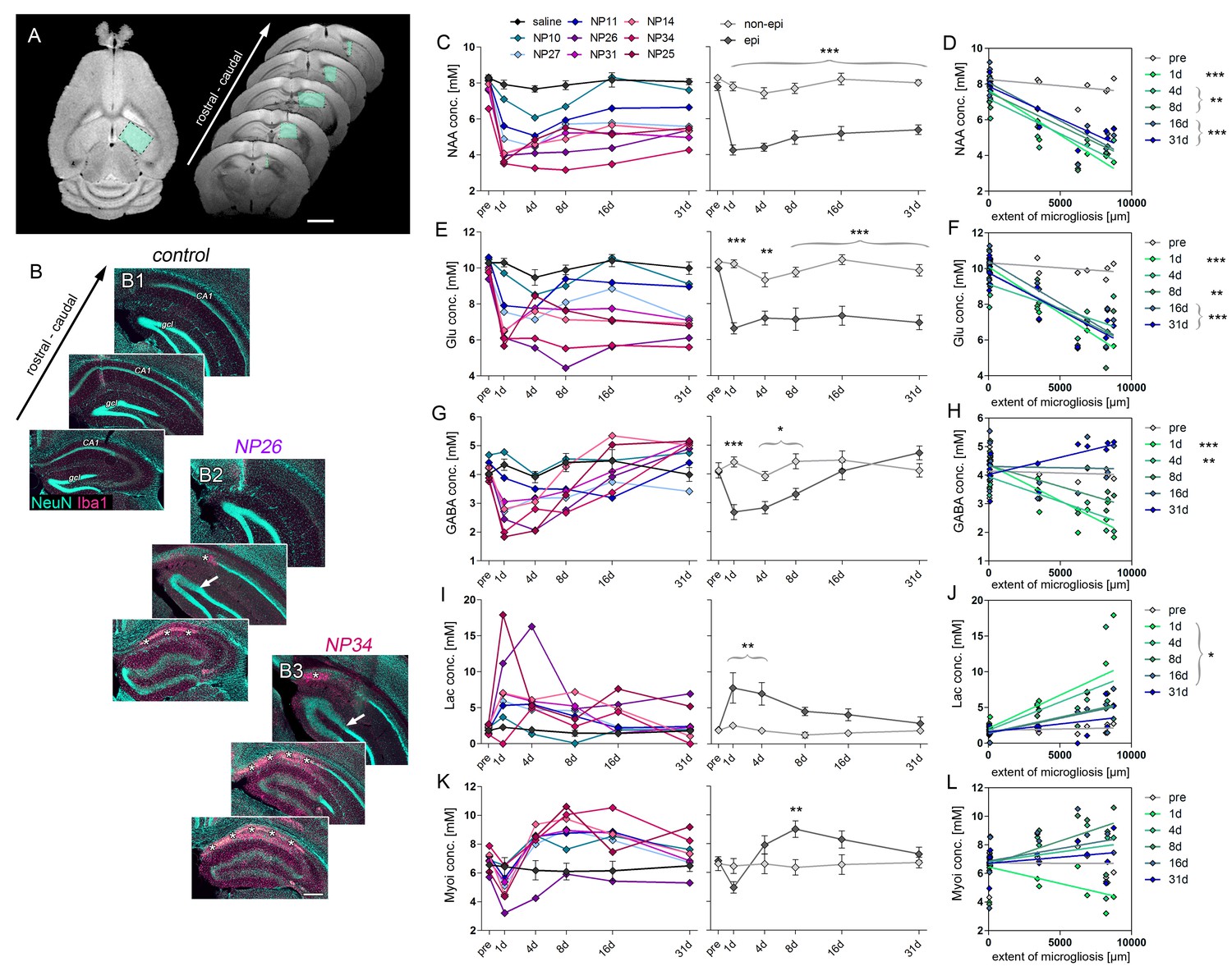
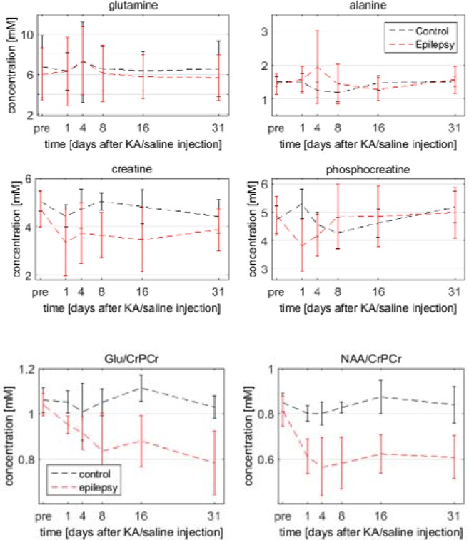
Early decline of glutamate and GABA predict HS.
(A) Representative horizontal and coronal T2 images illustrating the region-of-interest in the ipsilateral hippocampus (turquoise boxes) for 1H-MR-spectroscopy. N-acetyl aspartate (NAA) served as a marker for neurons. Glutamate (Glu) and gamma-aminobutyric acid (GABA) allowed to estimate the loss of excitatory and inhibitory neurons, respectively. Lactate (Lac) and myoinositol (Myoi) were used as surrogate markers for microglial and astroglial activation. (B) Representative photomicrographs of NeuN (turquoise, neurons) and Iba-1 (magenta, microglia) double-stained sections from one saline- (control) and two kainate-injected mice exhibiting different degrees of hippocampal sclerosis (NP26, moderate; NP34, strong) for qualitative comparison with the degree of metabolic alterations. Arrow, borders of the GCD; Asterisks, cell loss and microglial scarring in CA1. Scale bar in A, 2 mm; B, 200 µm. (C, E, G, I, K) Quantitative analysis of NAA, Glu, GABA, Lac and Myoi concentrations plotted for individual mice (left panel; controls, black, n = 5; kainate-injected animals color-coded) and groups (right panel; epileptic, dark grey; non-epileptic, light grey) during epileptogenesis. Source data is provided in ‘Figure 3—source data 1'. Two-way ANOVA; Bonferroni’s post-test; *p<0.05, **p<0.01, ***p<0.001; nnon-epi = 6, nepi = 7. Values are presented as the mean ± SEM. (D, F, H, J, L) Corresponding linear regression analysis of metabolite concentrations at distinct time-points during epileptogenesis (color-coded) with the extent of cell death-associated microgliosis in epileptic and non-epileptic mice (n = 13; Pearson’s correlation, corrected for multiple comparison; *p<0.05, **p<0.01, ***p<0.001).
-
Figure 3—source data 1
Summary of 1H-MR metrics.
Quantitative values of 1H-MR spectroscopy are listed for individual mice (saline-injected: N12, NP13, NP17, NP28, NP29; kainate-injected: NP10, NP11, NP14, NP25, NP26, NP27, NP31, NP34) and longitudinal time points (pre, 1d, 4d, 8d, 16d, 31d following injection).
- https://doi.org/10.7554/eLife.25742.010
Figure 4
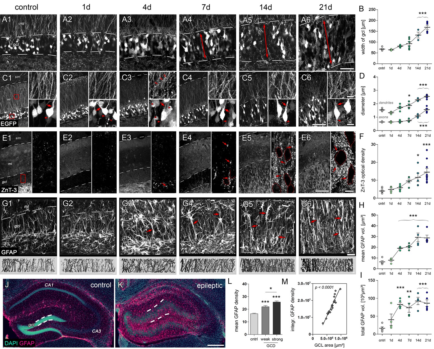
Microstructural alterations in the DG during epileptogenesis.
(A1-6 and C1-6) Representative confocal images show changes in the cytoarchitecture of the DG (double-headed arrows denote the dispersion of the GCL) and morphological features of individual eGFP-labeled granule cells, respectively (left panel: Overview; upper and lower right: High-magnification of granule cell dendrites or somata, respectively; red arrowheads, axon initial segments; red arrows, stem dendrites; red open arrows, dendritic swellings; red asterisks, degenerating granule cells. (B) Quantification of the GCL width (ncntrl = 7, n1d = 3, n4d = 5, n7d = 6, n14d = 3, n21d = 6) and (D) the diameter of initial axons and stem dendrites (ncntrl = 5, n1d = 3, n4d = 5, n7d = 4, n14d = 3, n21d = 5). (E1-6) Representative confocal z-plane images of ZnT-3 staining in the DG to determine the dynamics of mossy fiber sprouting (red arrows; ncntrl = 8, n1d = 4, n4d = 5, n7d = 5, n14d = 5, n21d = 9). Locations of granule cell somata are spared (dotted outlines). (F) Quantitative analysis of ZnT-3 optical density. (G1-6) Representative confocal images of GFAP-stained sections (upper panel) and corresponding 3D-reconstruction in the GCL (lower panel). h, hilus; gcl, granule cell layer; ml, molecular layer; slm, stratum lacunosum moleculare. (H–I) Quantitative analysis of the mean and total volume of GFAP-stained processes from radial glia cells in the GCL (ncntrl = 5, n1d = 4, n4d = 5, n7d = 4, n14d = 4, n21d = 5). All statistics were performed with one-way ANOVA, Dunnett’s post-test (compared to saline controls); *p<0.05, **p<0.01, ***p<0.001. (J, K) Representative sections stained for DAPI (turquoise) and GFAP (magenta) in controls and chronic epileptic mice (21d following kainate injection), respectively. Dashed lines denote the borders of the GCL. (L) Quantitative analysis for the optical density of GFAP in individual sections from three controls and in sections from three kainate-injected mice exhibiting weak and strong GCD (one-way ANOVA, Dunnett’s post-test; *p<0.05, **p<0.01, ***p<0.001; number of sections, ncntrl = 51, nw-GCD = 6, ns-GCD = 14). (M) Corresponding linear regression analysis for the integrated GFAP optical density and (I) the area of the GCL (Pearson’s correlation). Scale bars in A, 50 µm; in C (left), 100 µm; in C (right), 10 µm; in E (left), 100 µm; in E (right), 10 µm; in G, 30 µm; in K, 200 µm.
Figure 5 with 2 supplements
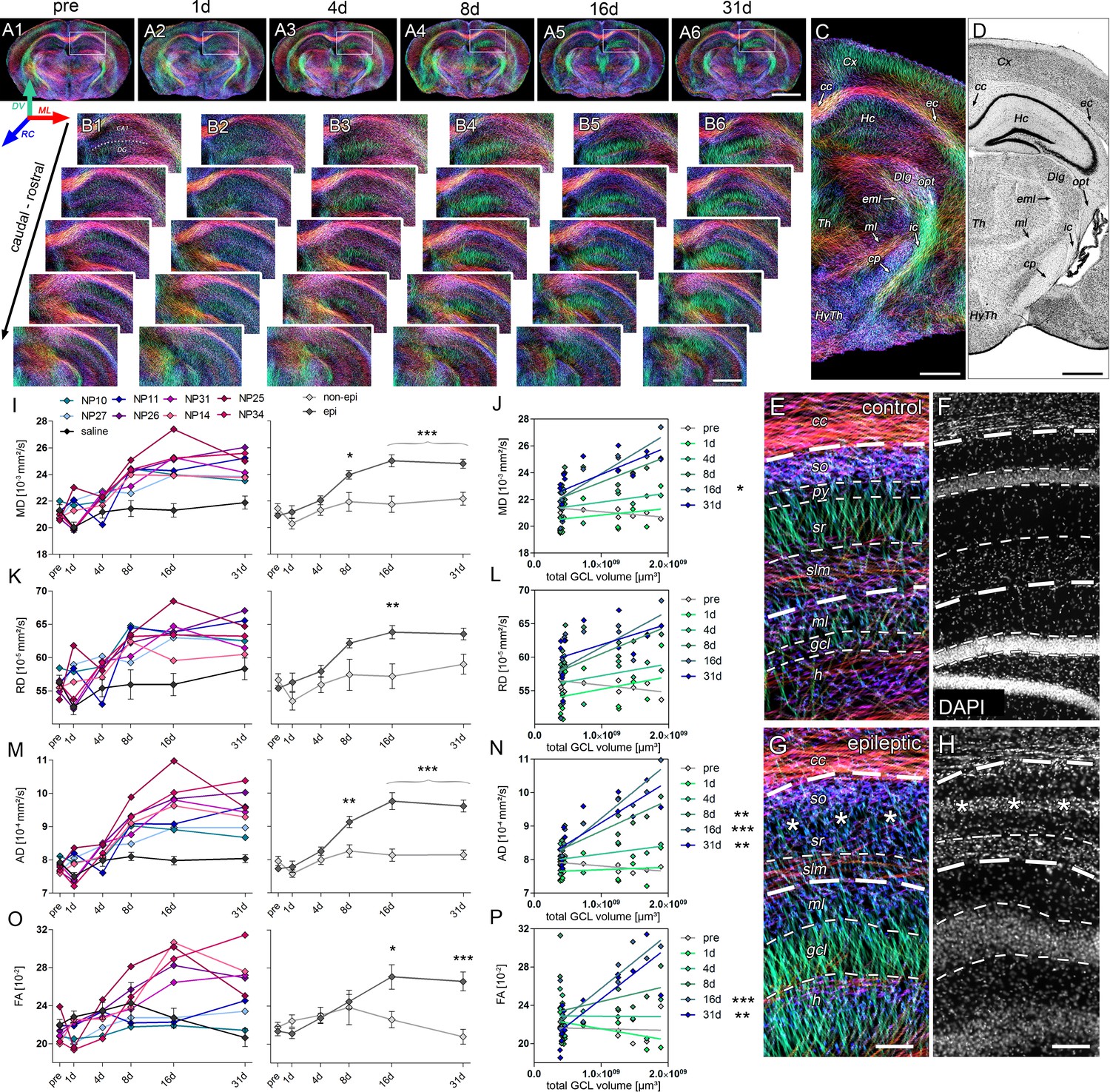
Microstructural reorganization quantified by DWI during epileptogenesis predicts disease progression.
(A1-6) Representative coronal sections from diffusion-weighted tractography at different time points during epileptogenesis (before injection = pre; 1d, 4d, 7d, 14d and 31d following SE). (B1-6) Enlarged images of the ipsilateral hippocampus at different levels along the rostro-caudal axis. The orientation of computed streamlines is color-coded [dorsoventral (DV), turquoise; mediolateral (ML), red; rostrocaudal (RC), blue]. (C–D) Representative tractography image and a Nissl-stained section (modified from Paxinos and Franklin, The Mouse Brain in Stereotaxic Coordinates, 2001) of corresponding brain regions for anatomical comparison. Computed fibers relate to major axonal pathways and brain regions exhibiting highly oriented dendrites (cc, corpus callosum; cp, cerebral peduncle; Cx, cortex; Dlg, dorsal lateral geniculate nucleus; ec, external capsule; eml, external medullary lamina; Hc, hippocampus; HyTh, hypothalamus; ic, internal capsule; ml, medial lemniscus; opt, optic nerve; Th, thalamus). (E, G) Enlarged tractography images demonstrating the distinct orientation of streamlines in different hippocampal layer (dashed lines; cc, corpus callosum; so, stratum oriens; py, pyramidal layer; sr, stratum radiatum; slm, stratum lacunosum moleculare; ml, molecular layer; gcl, granule cell layer; asterisks denote the region of pyramidal cell loss). (F, H) Corresponding DAPI-stained sections. Scale bars in A, 2 mm; B-D, 500 µm; H (left), 100 µm. (I, K, M, O) Quantitative analysis of DWI metrics [mean- (MD), radial (RD), axial diffusivity (AD) and fractional anisotropy (FA)] in the DG, plotted for individual mice (left panel; controls, black, n = 5; kainate-injected animals color-coded) and for groups (right panel; epileptic, dark grey; non-epileptic, light grey) during epileptogenesis. Source data is provided in ‘Figure 5—source data 1'. Two-way ANOVA, Bonferroni’s post-test, **p<0.01; ***p<0.001; nnon-epi = 6, nepi = 7. Values are presented as the mean ± SEM. (J, L, N, P) Corresponding linear regression analysis of DWI metrics at distinct time points during epileptogenesis with the total GCL volume in epileptic and non-epileptic mice (n = 13; Pearson’s correlation, corrected for multiple comparison; *p<0.05, **p<0.01, ***p<0.001). Refer to ‘Figure 5—figure supplement 1' for DWI metrics acquired in CA1.
-
Figure 5—source data 1
Summary of DWI metrics.
Quantitative values of DWI measurements are listed for individual mice (saline-injected: N12, NP13, NP17, NP28, NP29; kainate-injected: NP10, NP11, NP14, NP25, NP26, NP27, NP31, NP34) and longitudinal time points (pre, 1d, 4d, 8d, 16d, 31d following injection).
- https://doi.org/10.7554/eLife.25742.013
Figure 5—figure supplement 1

DWI changes in CA1 during epileptogenesis are poor predictors for hippocampal sclerosis.
(A, C, E, G) Quantitative analysis of DWI metrics in the CA1 region, plotted for individual mice (left panel; controls, black, n = 5; kainate-injected animals color-coded) and groups (right panel; epileptic, dark grey; non-epileptic, light grey) during epileptogenesis. Two-way ANOVA, Bonferroni’s post-test, *p<0.05; **p<0.01; nnon-epi = 6, nepi = 7. Values are presented as the mean ± SEM. (B, D, F, H) Corresponding linear regression analysis of DWI metrics at distinct time points during epileptogenesis with the extent of microglial scarring in the CA1 region of epileptic and non-epileptic mice (n = 13; Pearson’s correlation, corrected for multiple comparison; *p<0.05).
Figure 5—figure supplement 2
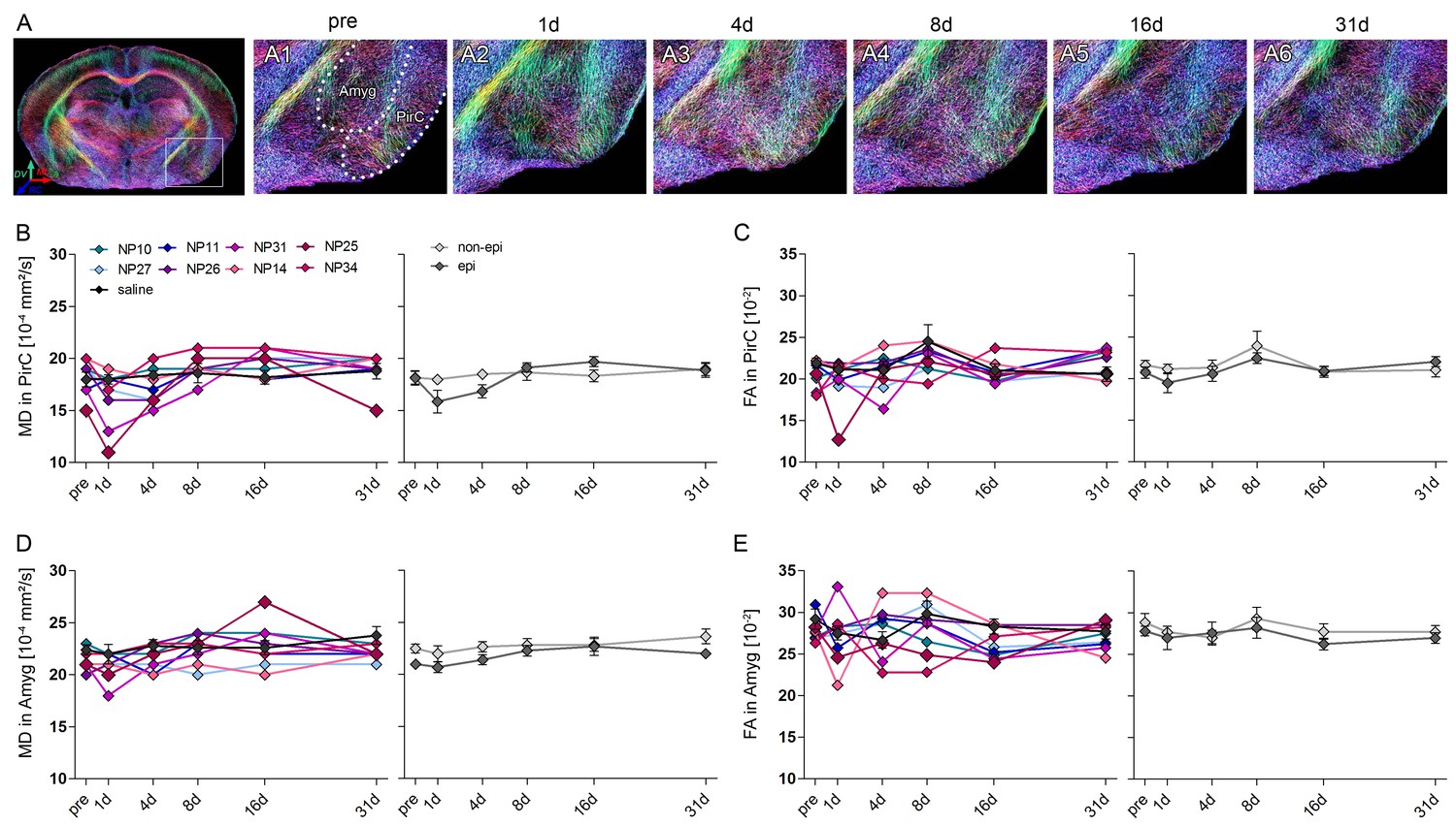
DWI changes in the piriform cortex and the amygdala during epileptogenesis.
(A) Representative coronal section of diffusion-weighted tractography images before injection. White box denotes the location of the amygdala (Amyg) and the piriform cortex (PirC). (A1-6) Enlarged tractography images of the piriform cortex (PirC) and the amygdala (Amyg) at different time points during epileptogenesis in the same animal (before injection, pre and 1d, 4d, 7d, 14d and 31d following SE). Scale bar: 50 µm. (B–E) Quantitative analysis of the mean diffusivity (MD) and fractional anisotropy (FA) in the piriform cortex and the amygdala, respectively. Values are plotted for individual mice (left panel; controls, black, n = 5; kainate-injected animals color-coded) and for groups (right panel; epileptic, dark grey; non-epileptic, light grey) during epileptogenesis. Two-way ANOVA, Bonferroni’s post-test, nnon-epi = 6, nepi = 7. Values are presented as the mean ± SEM.
Figure 6
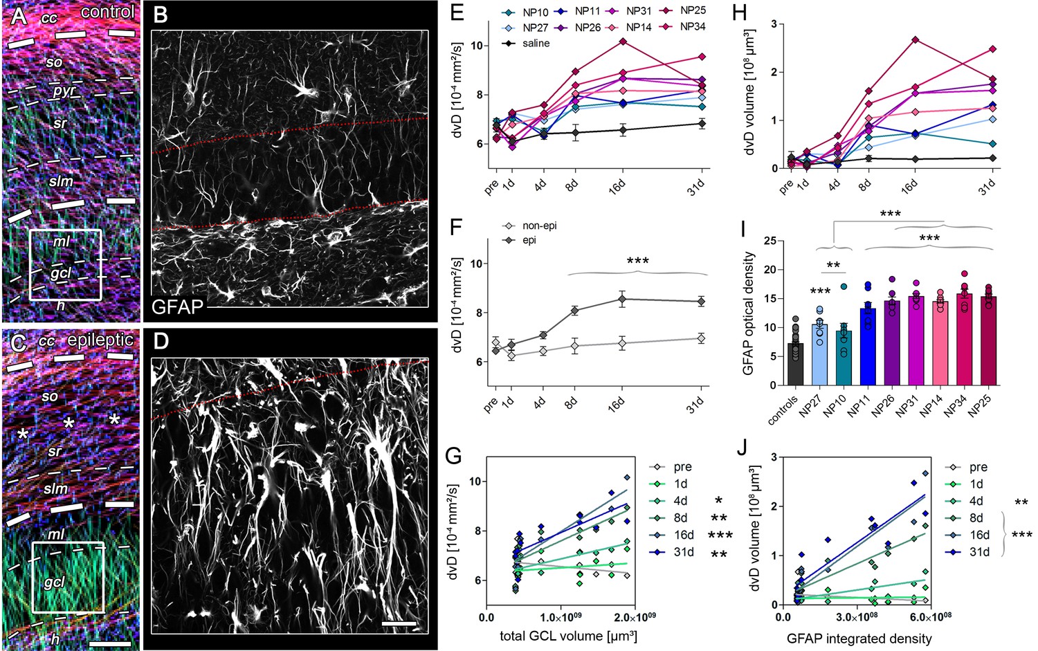
Radial gliosis contributes to DWI metrics.
(A, C) Representative DWI tractography maps of control and epileptic mice. Dashed lines, borders of the hippocampal layers; cc, corpus callosum; so, stratum oriens; py, pyramidal layer; sr, stratum radiatum; slm, stratum lacunosum moleculare; ml, molecular layer; gcl, granule cell layer. Scale bar, 100 µm. (B, D) High-magnification confocal images of GFAP staining in the region-of-interest corresponding to A and C (indicated as white boxes). Scale bar, 30 µm. (E, H) Quantitative analysis of dorsoventral diffusivity (dvD) in the DG and the calculated volume of increased dvD, respectively, plotted for individual mice (color-coded). (F) Groups analysis of dvD for epileptic (dark grey) and non-epileptic (light grey) during epileptogenesis. Source data is provided in ‘Figure 6—source data 1'. Two-way ANOVA, Bonferroni’s post-test, **p<0.01; ***p<0.001; nnon-epi = 6, nepi = 7. Values are presented as the mean ± SEM. (I) Quantitative analysis of GFAP optical density plotted for controls (black, n = 5) and individual kainate-injected mice (color-coded). One-way ANOVA, Bonferroni’s post-test, **p<0.01; ***p<0.001, number of sections, ncntr l= 40 (8 sections from five controls each), nNP10 = 8, nNP11 = 8, nNP14 = 8, nNP25 = 8, nNP26 = 8, nNP27 = 8, nNP31 = 8, nNP34 = 8. (G, J) Linear regression analysis of dvD and the calculated dvD volume at distinct time points during epileptogenesis with the total GCL volume and the integrated density of GFAP staining, respectively, in epileptic and non-epileptic mice (n = 13; Pearson’s correlation, corrected for multiple comparison; *p<0.05, **p<0.01, ***p<0.001).
-
Figure 6—source data 1
Summary of dorsoventral diffusivity metrics.
Quantitative values of dorsoventral diffusivity (dvD) measurements are listed for individual mice (saline-injected: N12, NP13, NP17, NP28, NP29; kainate-injected: NP10, NP11, NP14, NP25, NP26, NP27, NP31, NP34) and longitudinal time points (pre, 1d, 4d, 8d, 16d, 31d following injection).
- https://doi.org/10.7554/eLife.25742.017
Figure 7 with 2 supplements
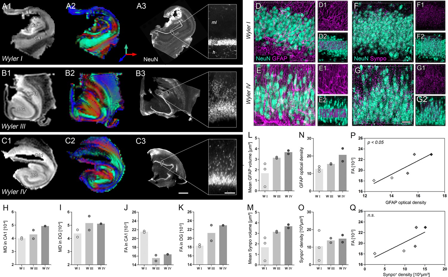
Validation of DWI biomarkers in human mTLE.
(A1–C1) T2-weighted images of sclerotic human hippocampi from mTLE patients scanned ex vivo. (A2–C2) Corresponding FA maps (color-coded for orientation: dorsoventral, turquoise; mediolateral, red; rostrocaudal: blue). Mean diffusivity (MD) and fractional anisotropy (FA) values for CA1 and DG are denoted in the lower-left, respectively. (A3–C3) Representative NeuN staining of scanned sections. Different Wyler grades according to the severity of neuronal loss (W I: mild, W III: moderate; W IV: strong). Scale bars, 3 mm; inset, 200 µm. (D–E) Representative confocal images of hippocampal sections (Wyler I and IV) double immunolabeled for NeuN (turquoise, neurons) and GFAP (magenta, astrocytes and radial glia cells) or (F–G) NeuN and Synaptoporin (magenta, mossy fiber synapses), respectively, revealing differences in the microstructure of the human DG between Wyler grades. (D1–E1, F1–G1) GFAP and Synaptoporin staining alone. (D2–E2, F1–G2) NeuN staining displayed together with reconstructed radial glia processes and mossy fiber boutons within the GCL, respectively. (H–I, J–K) Quantitative analysis for MD and FA in CA1 and in the DG, respectively (nWI = 2, nWIII = 2, nWIV = 1; no statistical test performed). Refer to ‘Figure 7—figure supplement 1' for MRI metrics acquired lower scanning resolution. (L) Quantitative analysis for the mean volume of GFAP-labeled radial glia processes as well as (M) Synaptoporin-labeled mossy fiber synapses, (N) and for GFAP optical density as well as (O) the density of Synaptoporin-labeled profiles within the GCL (nWI = 3, nWIII = 2, nWIV = 2; no statistical test performed). (P, Q) Correlation of FA values with the GFAP optical density and the density of Synaptoporin-labeled profiles, respectively (nWI = 2, nWIII = 2, nWIV = 1; Pearson’s correlation).
Figure 7—figure supplement 1
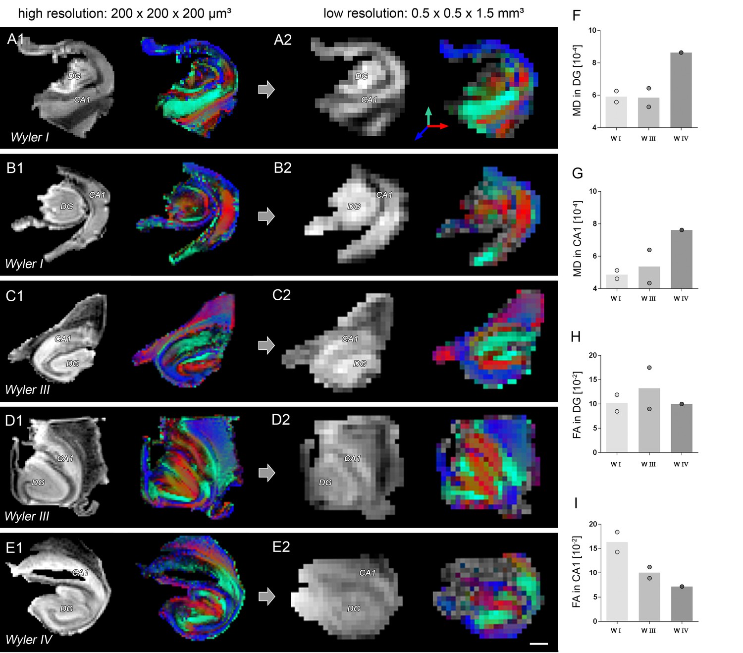
Comparison of high- and low-resolution ex vivo DWI.
(A1–E1) T2-weighted images and corresponding FA maps of human hippocampi from mTLE patients scanned ex vivo at high (200 × 200×200 µm³), and (A2–E2) at low resolution (0.5 × 0.5×1.5 µm³). FA maps are color-coded for orientation: dorsoventral, turquoise; medio-lateral, red; rostro-caudal: blue. (F–G, H–I) Quantitative analysis for mean diffusivity (MD) and fractional anisotropy (FA) in CA1 and in the DG at low scanning resolution. Scale bar: 2 mm.
Figure 7—figure supplement 2
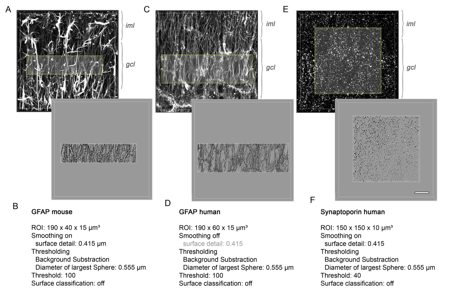
Imaris-based 3D-reconstruction.
(A) Volume-rendered confocal z-stack of GFAP staining in mouse (C) human, and (E) Synaptoporin in human DG (upper panel). Corresponding surface reconstruction of immunolabeled profiles within a region-of-interest in the GCL (lower panel). gcl, granule cell layer; iml, inner molecular layer. (B, D, F) List of parameters used for Imaris-based surface reconstruction.
Figure 8
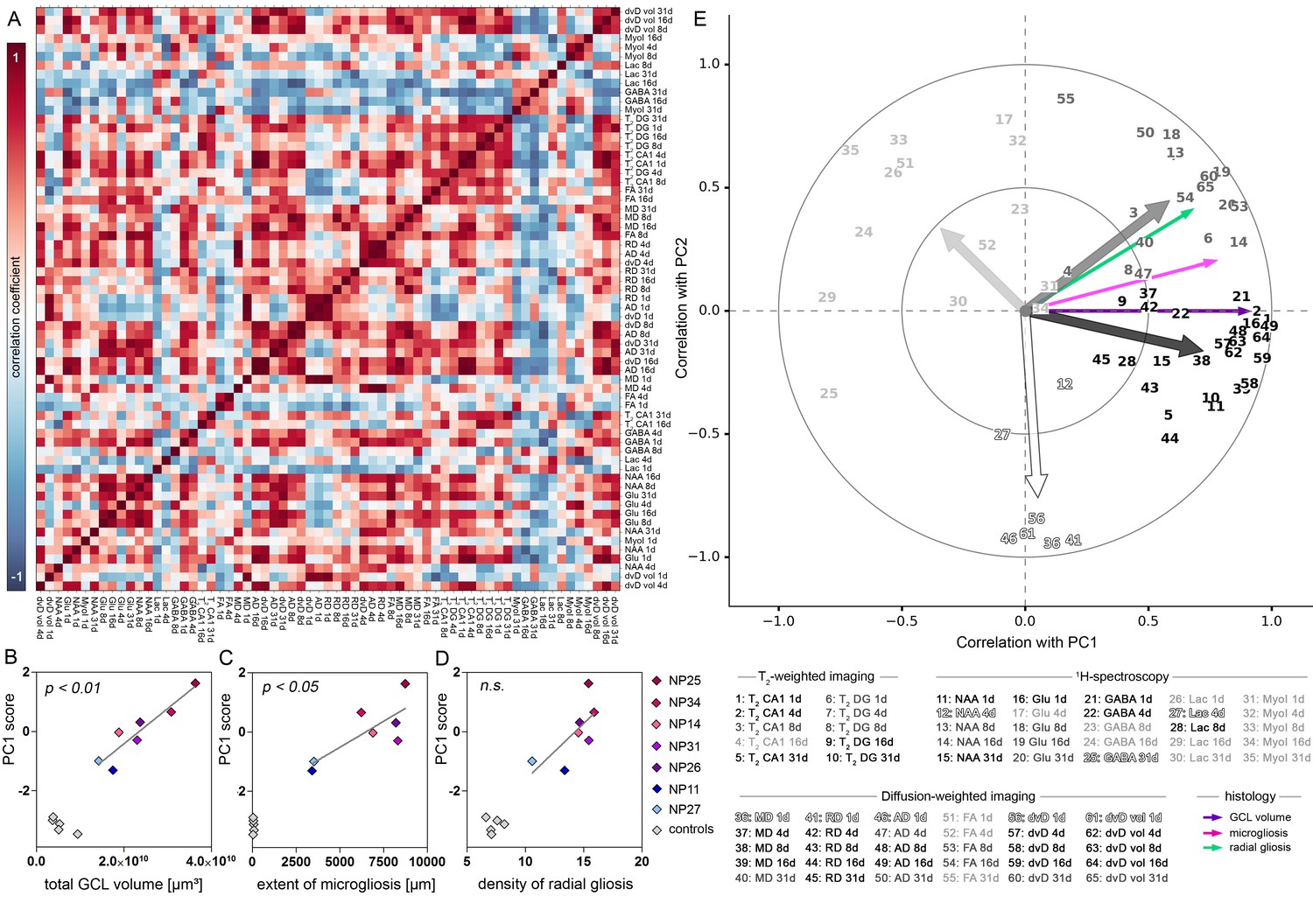
PCA-based evaluation of MRI biomarkers.
(A) Correlation matrix of imaging parameters used for PCA. Only data of kainate-injected mice was analyzed. Positive and negative correlation coefficients are color-coded in red and blue, respectively. (B) Pearson’s correlation analysis of PC1 scores and total GCL volume, (C) extent of microgliosis and (D) radial gliosis (i.e optical density of GFAP in the GCL) in epileptic mice (color-coded, n = 7). Controls (grey, n = 5) are plotted but not included in the analysis. (E) Correlation plot showing the similarity of individual MRI variables with PC1 and 2. Clusters of variables, indicated as numbers, are grey scale-coded. Arrows denote the population vector of the corresponding cluster. Coefficients are indicated as circles (small = 0.5; large = 1.0).
Figure 9 with 1 supplement
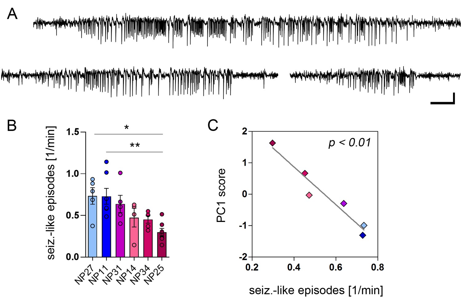
PCA-verified biomarkers predict the seizure severity.
(A) Representative EEG recordings from the ipsilateral hippocampus showing three examples of identified seizure-like episodes. Scale bars: Horizontal 5 s, vertical 2 mV. (B) Quantitative analysis of seizure-like episodes for individual epileptic mice (color-coded; note that EEG data is lacking for NP26). One-way ANOVA, Bonferroni’s post-test, *p<0.05, **p<0.01, number of recordings: nNP27 = 5, nNP11 = 7, nNP31 = 5, nNP14 = 4, nNP34 = 5, nNP25 = 7. Values are presented as the mean ± SEM. (C) Pearson’s correlation analysis of PC1 scores and the frequency of seizure-like episodes (n = 6).
Figure 9—figure supplement 1
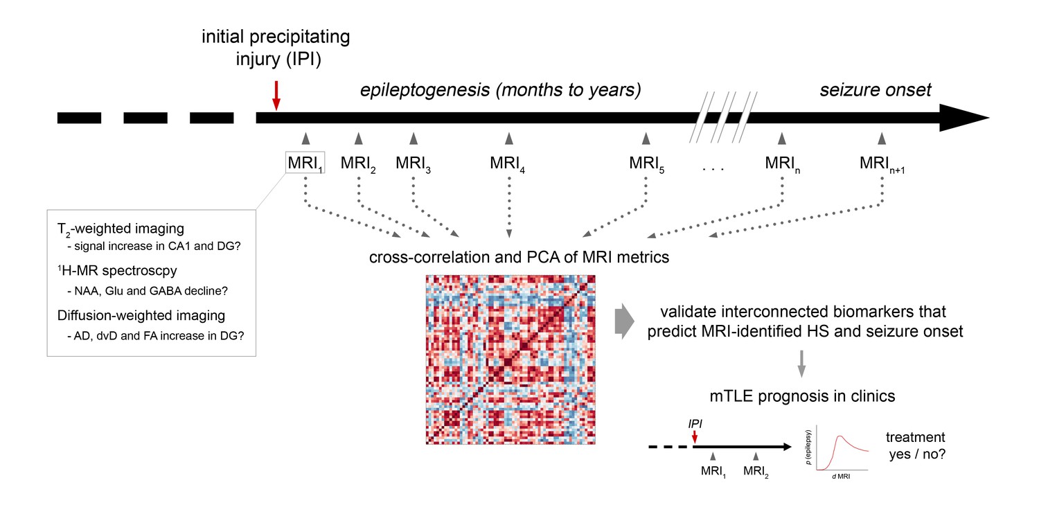
Experimental design to translate MRI biomarkers into the clinic.
Schematic illustrating an outline for the clinical translation of experimentally-identified biomarkers. Multimodal MRI is repeatedly applied early after the initial precipitating injury (IPI) until the onset of clinical seizures. Cross-correlation and PCA identifies interconnected MRI parameters and validates their predictive value with respect to MRI-identified HS and seizure onset in chronic mTLE. Subsequently, the change of MRI metrics (d) early after IPI can be assigned to the probability (p) of epilepsy onset and severity. Most robust MRI biomarkers can then be routinely used in clinics to prognose acquired mTLE, which allows to start anti-epileptogenic treatment early before clinical manifestation of epilepsy.
Author response image 1
Additional files
-
Supplementary file 1
Quantitative summary of statistically tested parameters.
The table displays all results statistical tests performed (right column) for each parameter (left column). The reference to the corresponding figure is given in the middle column. CI, confidence interval; n, number of animals; n*, number of sections; n°, number of recordings.
- https://doi.org/10.7554/eLife.25742.024
Download links
A two-part list of links to download the article, or parts of the article, in various formats.
Downloads (link to download the article as PDF)
Open citations (links to open the citations from this article in various online reference manager services)
Cite this article (links to download the citations from this article in formats compatible with various reference manager tools)
Early tissue damage and microstructural reorganization predict disease severity in experimental epilepsy
eLife 6:e25742.
https://doi.org/10.7554/eLife.25742


