Quantitative 3D-imaging for cell biology and ecology of environmental microbial eukaryotes
- Centre Nationnal de la Recherche Scientifique, France
- Université Pierre et Marie Curie, Sorbonne Universités, France
- European Molecular Biology Laboratory, Germany
- Paris Sciences et Lettres Research University, France
Figures
Figure 1 with 9 supplements
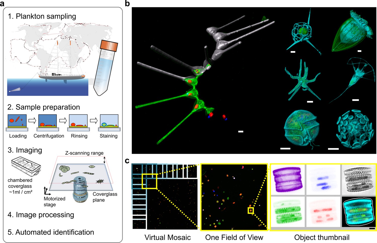
Environmental high-content fluorescence microscopy (e-HCFM): automated, 3D, and multichannel imaging for aquatic micro-eukaryotes.
(a) e-HCFM workflow applied to Tara Oceans samples: (1) 72 nano-plankton (size range 5–20 μm) samples collected during the Tara Oceans expedition (Pesant et al., 2015) were fixed in paraformaldehyde-glutaraldehyde buffer onboard and kept at 4°C for up to several years; (2) Samples were mounted in optical multiwell plates. Then, a 4-steps preparation allowed to stain all eukaryotic cells; (3) A commercial confocal laser scanning microscope was used to automatically image samples (40X NA1.1 water lens; 5 channels) generating 2.5 Tb of raw data (acquisition details in Figure 1—source data 1); (4) In total, 336,655 objects were processed for individual extraction of 480 descriptors (3D biovolumes, intensity distribution, shape descriptors and texture features, details in Figure 1—source data 2), and the reconstruction of various images for visual inspection (c); (5) A training set based on 18,103 manually curated images (5.4% of the dataset) classified into 155 categories, was used for automated recognition (Random Forest). (b) Examples of e-HCFM 3D-images and movies from a wide phylogenetic diversity of planktonic eukaryotes (see also Figure 1—figure supplements 1 and 2). Left panel: a chain of diatoms (Asterionellopsis sp., Heterokonta) (Figure 1—video 1); right panel, top left to bottom right: radiolarian (Rhizaria), ciliate (Alveolata), amoeba (Amoebozoa), choanoflagellate (Opisthokonta), dinoflagellate (Alveolata), coccolithophore (Haptophyta). Key cellular features are labelled with various dyes: DNA/nuclei (blue, Hoechst33342); (intra)cellular membranes (green, DiOC6(3)); cell covers and extensions (cyan, PLL-AF546, a home-made conjugation between α-poly-L-lysine (PLL) and Alexa Fluor 546 (AF546)); chloroplasts (red, chlorophyll autofluorescence). Scale bar 5 µm. (c) The confocal microscope is automated for acquiring multicolor Z-stacks over a mosaic of positions for each sample. Each field of view (fov) overlaps neighboring ones for detection of entire cells even if their position crossed one fov edge (see also Figure 1—figure supplement 4a). The imaging volume along the Z-axis comprises the space between the coverglass/sample interface plane and an upper limit corresponding to the theoretical thickest cell (Figure 1—figure supplement 3b). The fovs are then processed automatically and sequentially for detecting organisms without redundancy and for generating various images and Z-stack animations for visual inspection (Figure 1—videos 2 and 3).
-
Figure 1—source data 1
This image acquisition registry details the e-HCFM imaging runs, their metadata, their samples of origin, and associated metadata from the Tara Oceans expedition.
- https://doi.org/10.7554/eLife.26066.011
-
Figure 1—source data 2
List of descriptors computed for each object imaged through e-HCFM.
- https://doi.org/10.7554/eLife.26066.012
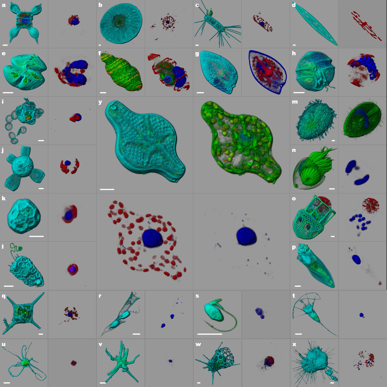
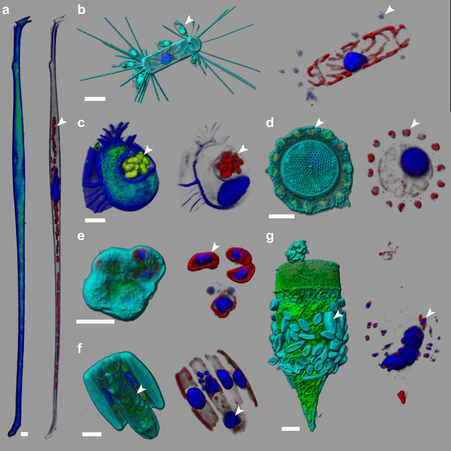
Figure 1—figure supplement 1
e-HCFM staining strategy is adapted to the environmental protistan biodiversity.
The samples (Tara Oceans expeditions) were fixed on board with a PFA-Glutaraldehyde buffer. They have been kept at 4°C for several years. The specimens were imaged manually from regular e-HCFM sample preparation with a Leica SP8 confocal laser scanning microscope (40X NA1.1 water). Four fluorescent channels were recorded: (i) Green, cellular membranes (DiOC6(3)) indicates the core cell bodies; DiOC6(3) also stains loricas of tintinnid ciliates (n, o); (ii) Blue, DNA (Hoechst) is used to localize DNA and nuclei; Hoechst may also stain the thecate dinoflagellate cell-wall (g); (iii) Red, chlorophyll (autofluorescence); (iv) Cyan, PLL-A546 is a useful counterstain for visualizing the specimen surface (This channel is omitted for specimen f, and n to display some specific membrane structures). All specimens are illustrated by two panels: the left side overlays all available fluorescent channels whereas the right side displays only the chlorophyll and the Hoechst fluorescence. The central inset (y) displays a diatom with four panels that peel off sequentially the four fluorescent channels available. The 3D reconstructions and volume rendering were conducted with the software Imaris (Bitplane, Switzerland). Scale bars are 5 µm. (a–d, y): five species of Bacillariophyta (diatoms). Planktoniella sp. cell (b) harbors small autotrophes on its surface. (e–h) four species of Holodinophyta (dinoflagellates). The specimen(f) illustrates the mixotrophy commonly found in this group. The ribbon shape chloroplasts surround the nucleus and the internal pusule (green volume on right-side panel) which shows the nucleus of a prey. (i–l): four species of Haptophyta (coccolithophores). (m–p): four species of Ciliophora (ciliates). m, a Colepidae specie; n-p, 3 Tintinnidae species. (q–t): various nano-flagellates. q, Dictyocha sp. (Dictyochophyceae); r, Dinobryon sp. (Chrysophyceae); s, unidentified specimen; t, unidentified Acanthoecid (choanoflagellate). (u–x): Various amoeboid protists. The first one (u) seems to harbor chloroplast-like structures. The second one (v) is heterotroph. There is one radiolarian (unidentified Nassellaria) with a fuzzy endosymbiont signal. The last one (x) is a foraminifera (unidentified Globigerin) housing endosymbiontic algae (red spots on the rightside panel).
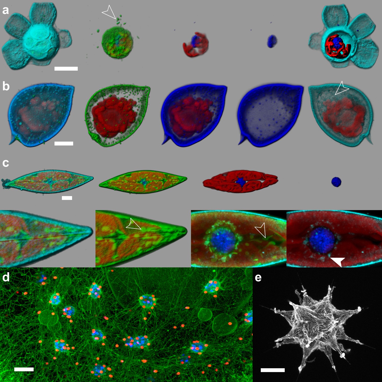
Figure 1—figure supplement 2
e-HCFM staining strategy is suitable for live imaging.
Four fluorescent channels were recorded: (i) Green, cellular membranes (DiOC6(3)) indicates the core cell bodies and organelles; (ii) Blue, DNA (Hoechst) is used to localize DNA and the nuclei; Hoechst may also stain the thecate dinoflagellate cell-wall (b); (iii) Red, chlorophyll (autofluorescence); (iv) Cyan/grey, PLL-A546 is a useful counterstain for visualizing the specimen surface (not visible in d). The 3D reconstructions and volume rendering were conducted with the software Imaris (Bitplane). (a) Scyphosphaera apsteinii (Roscoff Culture Collection, strain RCC 1455, Haptophyta, scale bar 10 µm). Few bacteria are hosted inside the barrel shape coccolithes (arrow head); (b) Prorocentrum micans (Roscoff Culture Collection, strain RCC 1517, Holodinophyta, scale bar 10 µm). This is a senescent specimen, membrane and nucleus are not properly stained, flagella is absent, and the PLL-A546 fully penetrated the cell (arrow head). Healthy dinoflagellates swim vigorously and cannot be imaged in 3D with CLSM. (c) Pleurosigma sp. (Roscoff Culture Collection, strain RCC 3090, Bacillaryophyta, scale bar 10 µm). This diatom shows some elongated mitochondria (arrow head). Additionally, PLL-A546 signal surrounds the nucleus in the endoplasmic reticulum (filled arrow head), suggesting internalization of the surface staining. (d) Colonial colodarian (environmental radiolarian, scale bar 100 µm). Each red sphere is an endosymbiontic dinoflagellate. Green digitations reticulate cytoplasm between the colony surface and the capsules where the nuclei are stored. Some vacuoles are visible. (e) Acantharian (environmental radiolarian, scale bar 50 µm). The PLL-A546 staining details the external membrane enveloping the cell. Both d and e specimens were collected at Villefranche-sur-Mer (France), Mediterranean sea.
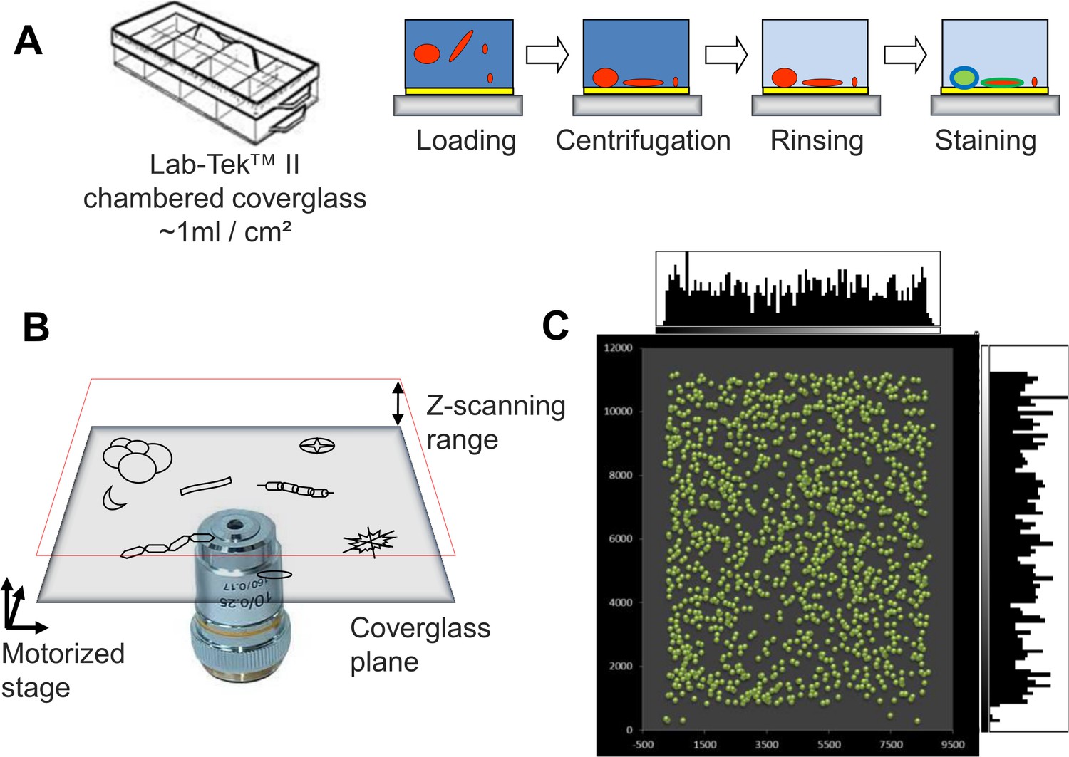
Figure 1—figure supplement 3
e-HTFM strategy for automated screening of planktonic protists.
(a) Sample preparation scheme (<1 hr). Concentrated cells from plankton samples are loaded into an eight-chamber Lab-TekTM II (Nunc 155382, Thermo Fisher Scientific, MA, USA) slide coated with poly-L-lysine, gently centrifuged and stained with three fluorescent dyes (Hoechst33342, DiOC6(3), poly-L-lysine-Alexa546). Only two rinsing steps are required for removing fixatives and for washing PLL-A546 dye. (b) The microscope stage is motorized in XYZ, allowing a fully automated positioning. After searching the glass/sample interface by a software autofocus, the image acquisition is conducted over a suitable Z-scanning range from the glass-bottom to the expected cell diameter. (c) After stitching together the fields of view covering the entire well bottom, particles were searched and their positions were plotted (green dots). Their distribution looks random and does not display obvious bias (lateral histograms quantify their distribution along X and Y axis).
Figure 1—figure supplement 4
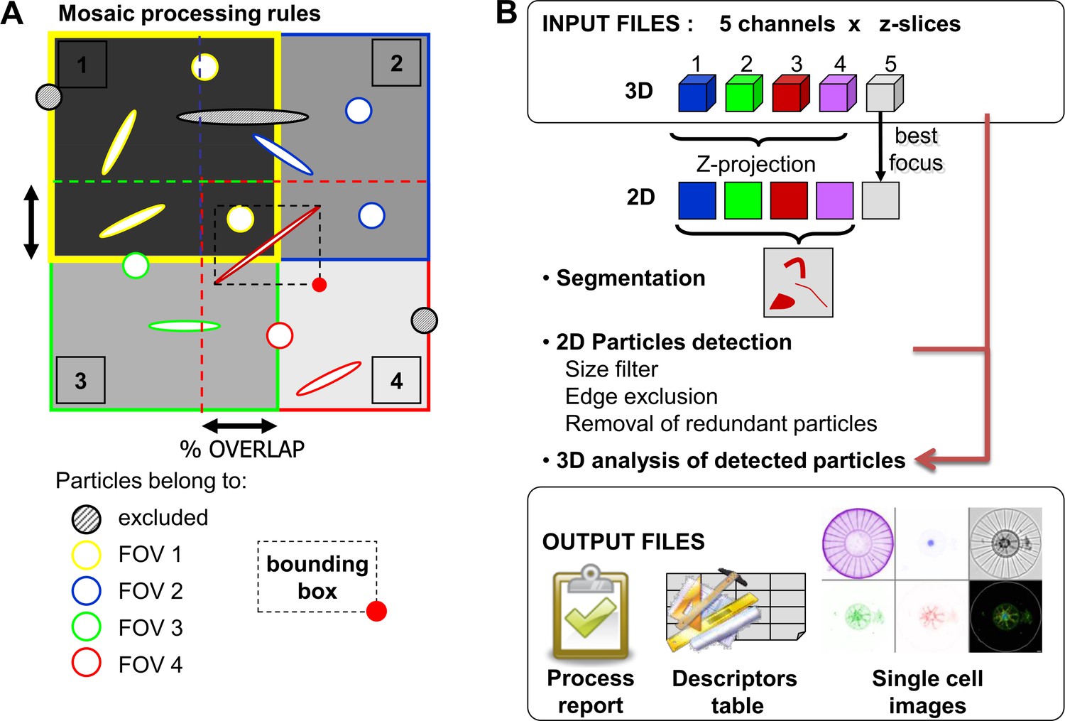
The image acquisition is coordinated with the image-processing strategy.
(a) Overlapping field of view (fov) reduces detection biases of large planktonic particles. The percentage of overlap between fovs is defined to fit the highest expected cell size. To avoid redundant detections cause by this overlapping, the fovs are processed successively (i.e. here 1 > 2 > 3 > 4) with the following rules: (i) a particle touching the edge of the analyzed fov is excluded; (ii) a particle belongs to a given field as far as the bottom right coordinates of its bounding box (red dot in field 4) do not belong to a previously analyzed fov. (b) Image processing pipeline was designed to: (i) segment particles; (ii) generate individual vignettes for experts’ recognition; and (iii) extract quantitative features from each particle. The segmentation is computed on the Maximum Intensity Projection (MIP) merging the MIP of each fluorescent channel z-stack (1, channel Hoechst; 2, Channel DiOC6; 3, channel Chlorophyll; 4, channel Alexa546; 5, transmitted light). Some filtering operations aim at excluding detected particles from the downstream analysis if they are smaller than a given the size threshold, or if they are touching the edge of the fov, or if they have been previously detected (see (a) above). The measurements are collected from 2D projections and 3D datasets and compiled in a single output file. A report summarizes the processing parameters, key steps and few calculations (e.g. particle concentration). The particle thumbnail is a montage of the cropped MIP from all but transmitted light channel, which is illustrated by the plane optimizing sharpness. The mask outline is also included for confirming the segmentation efficiency. A 5 µm scale bar is stamped onto the vignette.
Figure 1—figure supplement 5
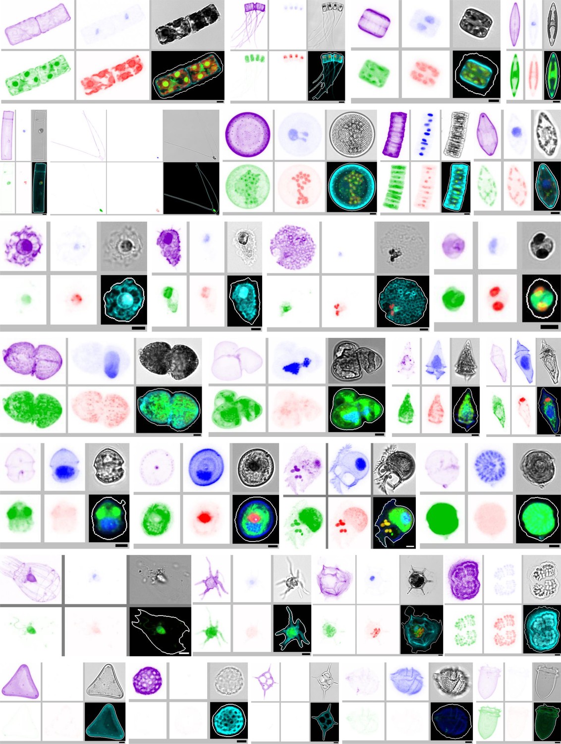
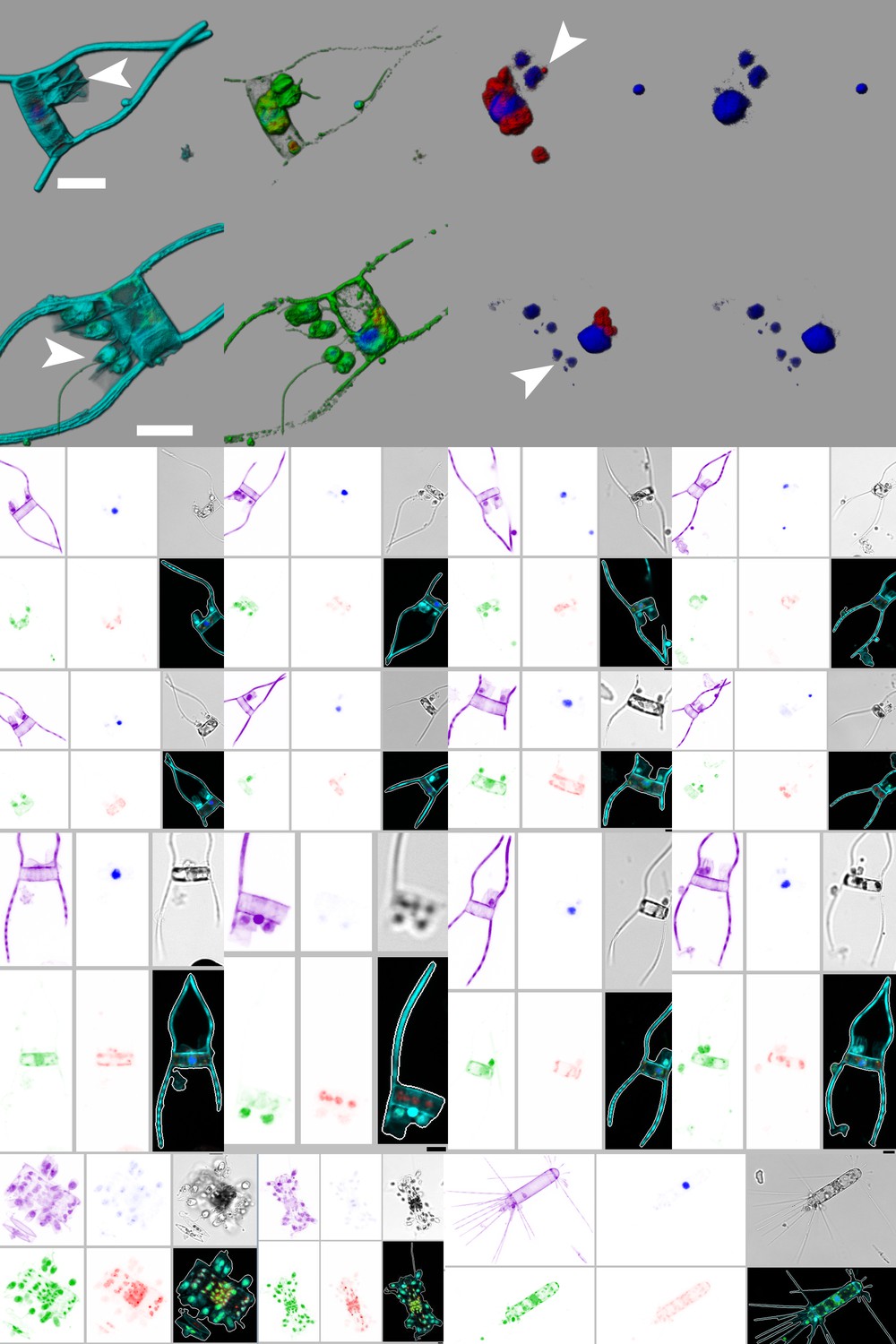
A short selection of the biodiversity that was detected by e-HCFM into 5–20 µm samples from the Tara Oceans expeditions.
Alexa-PLL staining clearly improved the full detection of almost all cells and specifically of their extensions and transparent biomineral structures (e.g. diatoms). The staining intensity is clearly variable according to the surface chemical properties of each cell type. The rows show: 1 and 2, diatoms (Bacillariophyta); 3, Coccolithophoridae (Haptophyta); 4 and 5, dinoflagellates (Holodinophyta); 6, few other lineages; 7, Few examples illustrate the efficient discrimination of ‘empty ‘cell envelope (no core cell structures) which cannot be mistaken with viable organisms. The scale bar is 5 µm; Blue, channel Hoechst; green, Channel DiOC6; red, channel Chlorophyll; purple, channel Alexa546; grey, bright field.
Figure 1—figure supplement 6
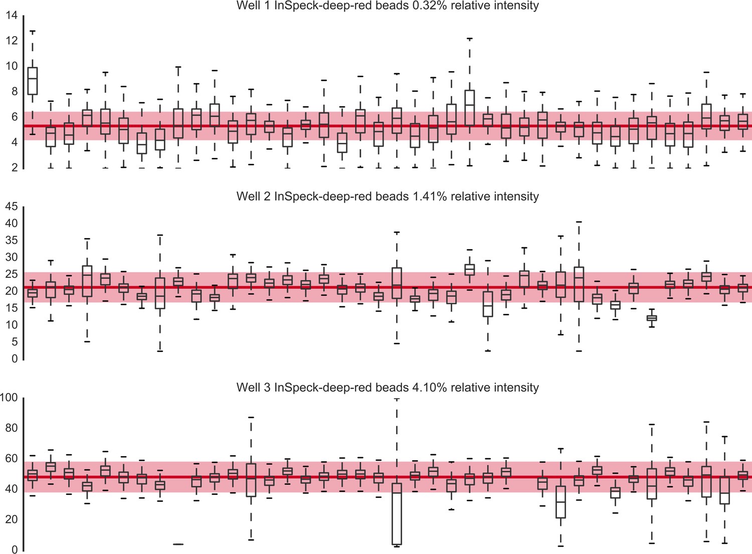
Monitoring the microscope performance over time by measuring the fluorescence intensity of three red fluorescing beads (Inspeck deep red 0.32% [top panel]; 1.41% [middle panel]; 4.10% [lower panel], I-7225, Invitrogen) in the chlorophyll channel (ex633/em680-700).
Each column represents one acquisition (in chronological order; acquisition spans a 10-month period) and the y-axis indicates the intensity value of voxels inside the bead (the data for each acquisition is summarised as a boxplot). The thick red line indicates the median intensity value and the shading denotes the region 20% below and 20% above the median. Source data are available in the file Figure 1—figure supplement 6—source data 1.
-
Figure 1—figure supplement 6—source data 1
Bead intensities for each bead.
This is the source data for Figure 1— figure supplement 6.
- https://doi.org/10.7554/eLife.26066.010
Figure 1—video 1
3D-animation of a Diatom (Asterionellopsis sp.) which illustrates the synergy between e-HCFM staining strategy and optical sectioning microscopy (CSLM).
The specimen (surface water, Tara Ocean station 72) was imaged manually from regular e-HCFM sample preparation with a Leica SP8 confocal laser scanning microscope (40X NA1.1 water). Four fluorescent channels are recorded: (i) Green: cellular membranes (DiOC6(3)) indicate the core cell bodies; (ii) Blue: DNA (Hoechst) is used to identify the nucleus; (iii) Red: chlorophyll (autofluorescence); (iv) Grey: PLL-Alexa546 is a useful counterstain for visualizing the specimen surface. 3D reconstruction, surface rendering and animation were conducted with the software Imaris (Bitplane).
Figure 1—video 2
First example of Z-stack animations that e-HCFM method provides for each detected organism (a chain of diatoms).
https://doi.org/10.7554/eLife.26066.014
Figure 1—video 3
Second example of Z-stack animations that e-HCFM method provides for each detected organism (a choanoflagellate).
https://doi.org/10.7554/eLife.26066.015
Figure 2 with 2 supplements
e-HCFM-staining strategy is effective in revealing symbiotic interactions in marine protists.
These seven cells, fixed on board Tara and kept at 4°C for several years, were imaged manually using the e-HCFM workflow (Figure 1). Each cell is illustrated by two panels: the left side overlays all available fluorescent channels whereas the right side displays only the chlorophyll and the Hoechst fluorescence. Four fluorescent channels were recorded: (i) Green: cellular membranes (DiOC6(3)) indicate the core cell bodies; it also stains loricas of tintinnid ciliates (g); (ii) Blue: DNA (Hoechst) identifies nuclei; it also stains the cell-wall of thecate dinoflagellate (a, c); (iii) Red: chlorophyll autofluorescence resolves chloroplasts; (iv) Cyan: PLL-A546 is a generic counterstain for visualizing eukaryotic cells’ surface (not used in a, (c). 3D reconstructions were conducted with the software Imaris (Bitplane). Scale bar is 10 µm. (a) Association between the heterotrophic dinoflagellate Amphisolenia and unidentified cyanobacteria hosted inside the cell wall (arrow head). (b) The diatom Corethron sp. (Figure 2—video 1) harbors several epiphytic nanoflagellates living in small lorica and attached onto the diatom frustule (arrow head). These have been observed in association with different diatom species (see Figure 2—figure supplement 1). (c) The dinoflagellate Citharistes sp. has developed a chamber (phaeosome) for housing cyanobacteria (arrow head). (d) The diatom Thalassiosira sp. is surrounded by a belt chain of 14 coccolithophores (Reticulofenestra sessilis, arrow head). (e) A juvenile pelagic foraminifer hosts endosymbiotic microalgae (arrowhead), likely Pelagodinium dinoflagellates. (f) Colonies of Fragillariopsis sp. diatoms are regularly observed in close interaction with tintinnid Salpingella sp. ciliate (arrowhead). The tintinnid lorica is inserted inside the groove of the barrel formed by the diatom chain. (g) The lorica of the ciliate Tintinnopsis sp. aggregates several epiphyte pennate diatoms, which were still alive prior to fixation as chloroplast and nuclei are visible (arrow head).
Figure 2—figure supplement 1
e-HCFM reveals an unreported epibiose involving the diatom Chaetoceros simplex and an unidentified nano-flagellate from the 5–20 µm samples of the Tara Oceans expeditions.
The two first rows of the plate illustrate how the epiphytic nano-flagellate cells are attached on the diatom frustule. They live in small tubes (lorica) which are bound at the base of the setae (arrow head, scale bar is 10 µm). Their DNA signature indicates additional signal surrounding the nucleus, which suggest DNA from prey and a heterotrophic behavior. The rows 3 to 5 display few examples of this interaction that were automatically identified by supervised machine learning (Figure 3—source data 1) with a recall value of 88.5% (46 specimens were positively classified from 52 specimens in the learning set and six were false positives from the 18051 other specimens in the learning set). We also provide in the row six few examples of similar associations involving other diatom species (see also Figure 2b). Blue, channel Hoechst; green, Channel DiOC6; red, channel chlorophyll; cyan/purple, channel Alexa546; grey, bright field.
Figure 2—video 1
3D-animation of a Diatom (Corethron sp.) which illustrates how the e-HCFM method supports investigation about microbial interactions.
The specimen (surface water, Tara Ocean station 137) was imaged manually from regular e-HCFM sample preparation with a Leica SP8 confocal laser scanning microscope (40X NA1.1 water). Four fluorescent channels are recorded: (i) Green: cellular membranes (DiOC6(3)) indicate the core cell bodies; (ii) Blue: DNA (Hoechst) is used to identify the nucleus; (iii) Red: chlorophyll (autofluorescence); (iv) Grey: PLL-Alexa546 is a useful counterstain for visualizing the specimen surface. 3D reconstruction, surface rendering and animation were conducted with the software Imaris (Bitplane).
Figure 3 with 4 supplements
Analysis of e-HCFM images and their descriptors.
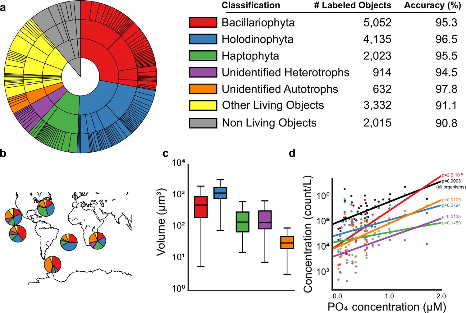
(a) Overview of the training set as a hierarchical pie chart. The size of the slices scales with the number of elements in the training set (details in Figure 3—source data 1). Accuracy values (%) show the recall for each of the 5-high level groupings considered (see also Figure 3—figure supplements 1, 2 and 4 and Figure 3—source data 1 and 2). (b) Relative abundances of recovered ‘live’ cells (cells with preserved organellar content, see Figure 1—figure supplement 5), per high-level group and per ocean basin (see also Figure 3—figure supplement 3, and Figure 3—source data 3 and 4). (c) Distribution of total cell biovolumes stratified per major taxonomic group. (d) Relationship between phosphate concentration and plankton concentration (in counts per liter); black line: total concentration of living organisms in the sample; colored line: total concentration in that taxonomic group (displayed p-values are Spearman correlations, lines are least-squares best-fits, see Methods and Figure 3—source data 5–7). [For reviewers - list of information supplements and legends]. (Tables cannot be included in the manuscript and they are provided as separated files).
-
Figure 3—source data 1
Organization of the hierarchical classification scheme for the automated classification, the training set categories abundance and the recall value for each category of the four levels (four tables).
- https://doi.org/10.7554/eLife.26066.028
-
Figure 3—source data 2
Confusion matrix generated by the classifier at the classification level 4.
- https://doi.org/10.7554/eLife.26066.029
-
Figure 3—source data 3
Relative abundance of each taxon in each sample.
The relationship between sample label and sampling location is provided in ‘Figure 1—source data 1.’.
- https://doi.org/10.7554/eLife.26066.030
-
Figure 3—source data 4
Assignment of stations to oceanic provinces.
- https://doi.org/10.7554/eLife.26066.031
-
Figure 3—source data 5
Object counts (normalized to seawater volume) per taxonomic group (panel d).
- https://doi.org/10.7554/eLife.26066.032
-
Figure 3—source data 6
Measured PO₄ concentrations (panel d).
- https://doi.org/10.7554/eLife.26066.033
-
Figure 3—source data 7
Values of N, Spearman correlation (rho), and number of samples (N) for each sub-group (panel d).
- https://doi.org/10.7554/eLife.26066.034
Figure 3—figure supplement 1
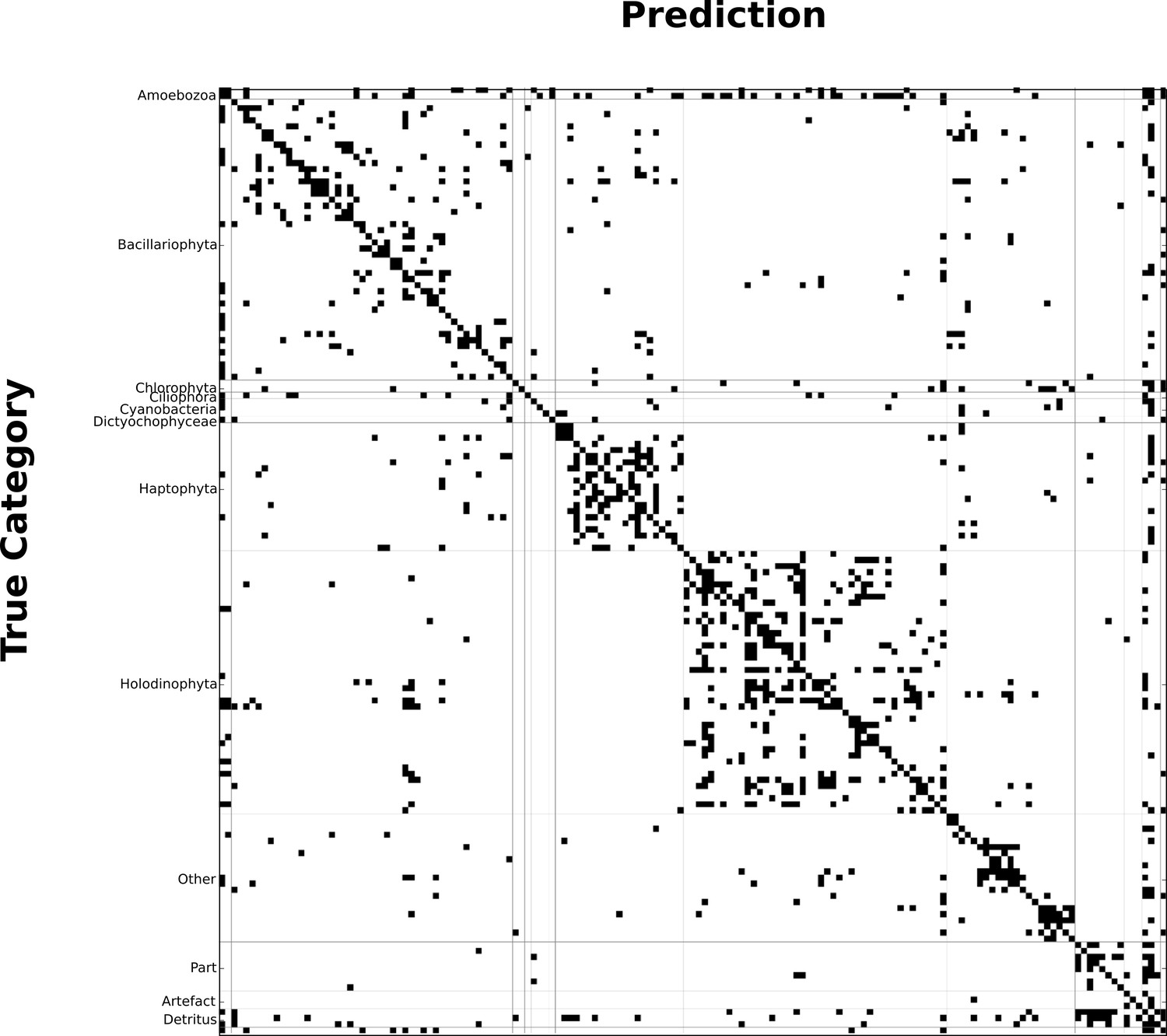
Binary confusion matrix showing how classification errors are typically within the same broad taxonomical group.
Both rows and columns represent the 155 categories. Cells are filled in whenever there is at least one labeled object of the category indicated in the row classified into the category indicated by the column (i.e., off-diagonal elements represent errors). Source data are available in the file Figure 3—source data 2.
Figure 3—figure supplement 2
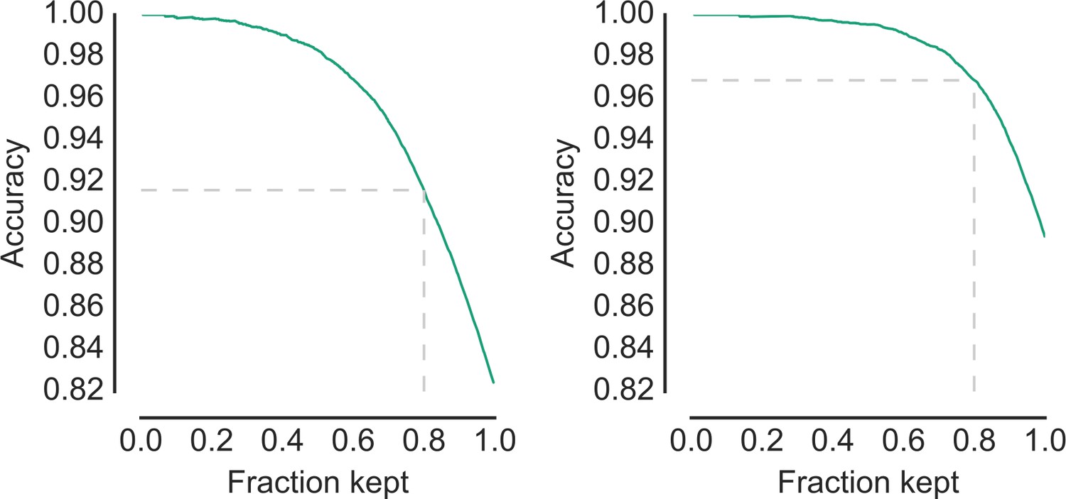
Tradeoff between accuracy and recall.
Shows the accuracy as a function of the fraction of high-confidence objects that are kept, results are displayed at the most-detailed, fourth level (left, 155 categories) or the intermediate third level (right, 33 categories) of the classification hierarchy. Dotted lines indicate the point at which 80% of the data points are kept. Source data are available in the files Figure 3—figure supplement 2—source data 1 (left panel) and Figure 3—figure supplement 2—source data 2 (right panel).
-
Figure 3—figure supplement 2—source data 1
Classification results for all objects in the training data at the fourth (finest) resolution level presented in in left panel (obtained by cross-validation).
- https://doi.org/10.7554/eLife.26066.022
-
Figure 3—figure supplement 2—source data 2
Classification results for all objects in the training data at the third resolution level presented in right panel (obtained by cross-validation).
- https://doi.org/10.7554/eLife.26066.023
Figure 3—figure supplement 3
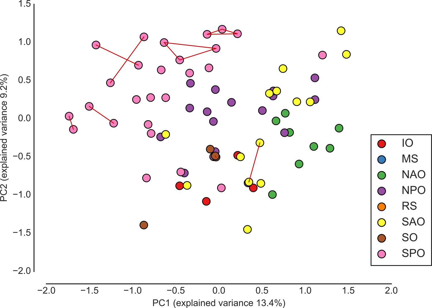
Ordination of eHCFM-derived taxonomic abundances reveals regional clustering and tests technical reproducibility of eHCFM-taxonomic profiling.
Principal component analysis of relative abundances of living single cells. Colors indicate ocean basin (IO: Indian Ocean, SAO: South Atlantic Ocean, SO: Southern Ocean, SPO: South Pacific Ocean, NPO: North Pacific Ocean, NAO: North Atlantic Ocean). Lines connect samples which were imaged in more than one run (technical replicates). Samples with fewer than 100 cells were excluded. Source data are available in the files Figure 3—source datas 3 and 4, and Figure 3—figure supplement 3—source data 1.
-
Figure 3—figure supplement 3—source data 1
Derived principal component values (original data is Figure 3—source data 2).
- https://doi.org/10.7554/eLife.26066.025
Figure 3—figure supplement 4
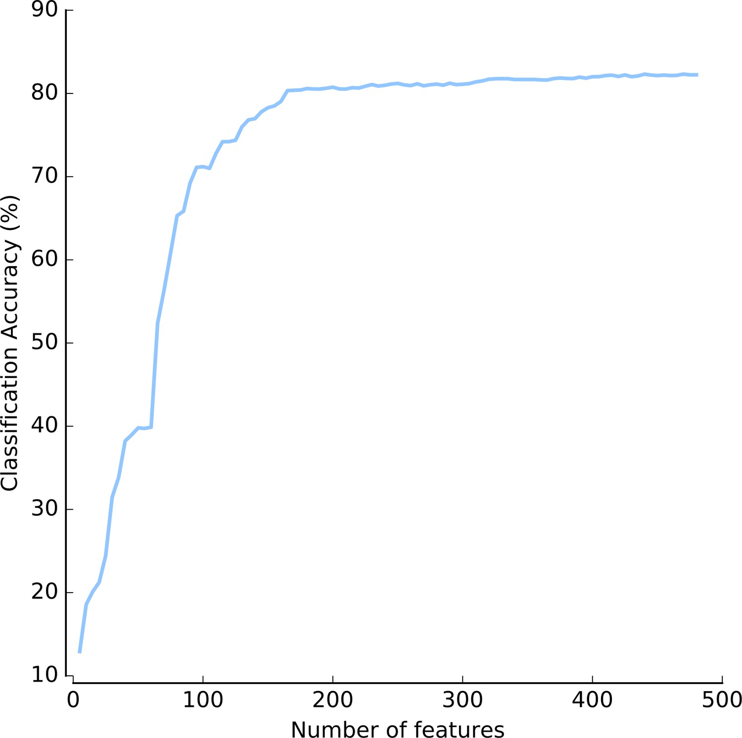
Classification accuracy as a function of the number of features.
Accuracy was estimated by cross-validation, using a feature selection step prior to classification. Source data are available in the file Figure 3—figure supplement 4—source data 1.
-
Figure 3—figure supplement 4—source data 1
Accuracy of classification (estimated by cross validation) using a limited number of features (from 5 to 480, in increments of 5).
- https://doi.org/10.7554/eLife.26066.027
Additional files
-
Transparent reporting form
- https://doi.org/10.7554/eLife.26066.035
Download links
A two-part list of links to download the article, or parts of the article, in various formats.
Downloads (link to download the article as PDF)
Open citations (links to open the citations from this article in various online reference manager services)
Cite this article (links to download the citations from this article in formats compatible with various reference manager tools)
Quantitative 3D-imaging for cell biology and ecology of environmental microbial eukaryotes
eLife 6:e26066.
https://doi.org/10.7554/eLife.26066


