Figures and data in Learning multiple variable-speed sequences in striatum via cortical tutoring | eLife

8 figures

Figures

Figure 1

Download asset Open asset

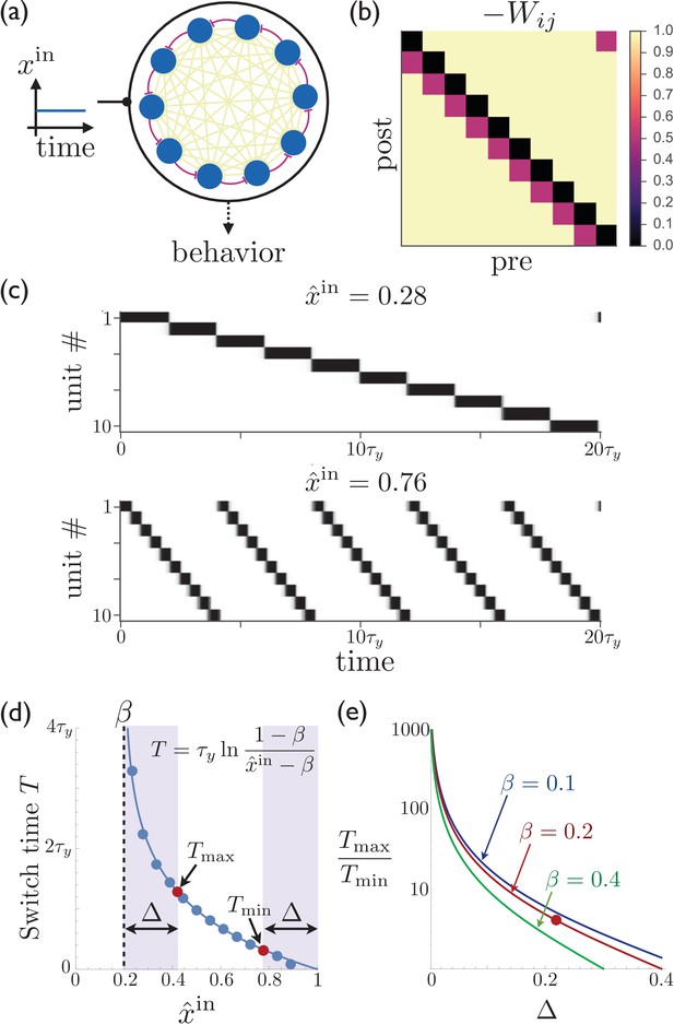
Rescalable sparse sequential activity in the striatum.

(a) Schematic diagram of a 10-unit striatal network. Units receive constant external excitatory input and mutually inhibit each other. The burgundy synapses correspond to a depotentiated path through the network that enables sequential activity. (b) The synaptic weight matrix for the network shown in ‘a’, with subdiagonal weights depotentiated by $η = 0.2$ . (c) The magnitude of the constant input $x^{in}$ to the network can be used to control the rate at which the activity switches from one population to the next. The units in the network are active in sequential order, with the speed of the sequence increasing as the excitatory input to the network is increased. Parameters for the synaptic depression are $β = 0.2$ and $τ_{y} = 20 τ$ , the gain parameter is $λ = 20$ , synapses connecting sequentially active units are depotentiated by $η = 0.1$ , and the effective input is ${\hat{x}}^{in} \equiv x^{in} / (1 - η)$ . (d) The switch time as a function of the level input to the network. Points are determined by numerically solving Equation 1; curve is the theoretical result (equation shown in figure; see Appendix 1 for details). If the input is limited to the range $β + Δ \leq {\hat{x}}^{in} \leq 1 - Δ$ (e.g. because reliable functioning in the presence of noise would require the input to stay away from the boundaries within which switching occurs), then $T_{\max}$ and $T_{\min}$ are the maximum and minimum possible switching periods that can be obtained. (e) The temporal scaling factor is shown as a function of $Δ$ for different values of the synaptic depression parameter $β$ . The red dot corresponds to the ratio of the red dots in ‘d’.

https://doi.org/10.7554/eLife.26084.002

Figure 2

Download asset Open asset

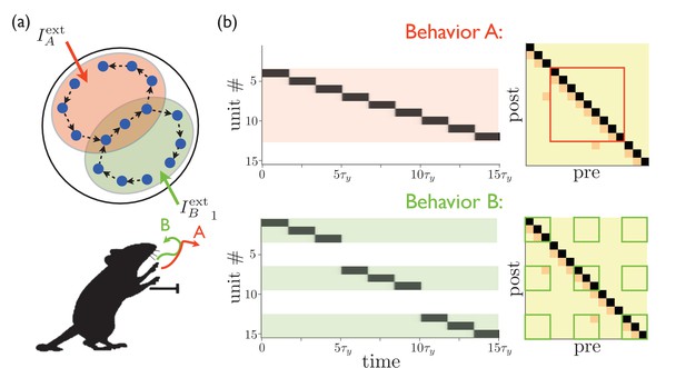
Targeted external input expresses one of several sequences.

(a) Schematic illustration of partially overlapping striatal activity sequences selectively activated by external input. The arrows do not represent synaptic connections, but rather the sequence of activity within an assembly. Overlapping parts of the striatal activity sequences encode redundancies in portions of the corresponding behaviors (in this case, the middle portion of a paw movement trajectory). (b) Left panels show network activities in which only the shaded units receive external input. Right panels show the weights, with only the outlined weights being relevant for the network dynamics for each behavior.

https://doi.org/10.7554/eLife.26084.003

Figure 3

Download asset Open asset

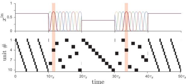
Driving the network from Figure 1 with two different types of input leads to distinct operational modes.

If input to the network (top) is tonic, the recurrent weights cause the network to produce a particular activity sequence (bottom), as in Figure 1, with the magnitude of the input controlling the speed of the sequence. Alternatively, if the input is strongly time-dependent, then the network dynamics are enslaved to the input pattern. In this case each unit receives a unique pulsed input, with the input to unit four highlighted for illustration.

https://doi.org/10.7554/eLife.26084.004

Figure 4

Download asset Open asset

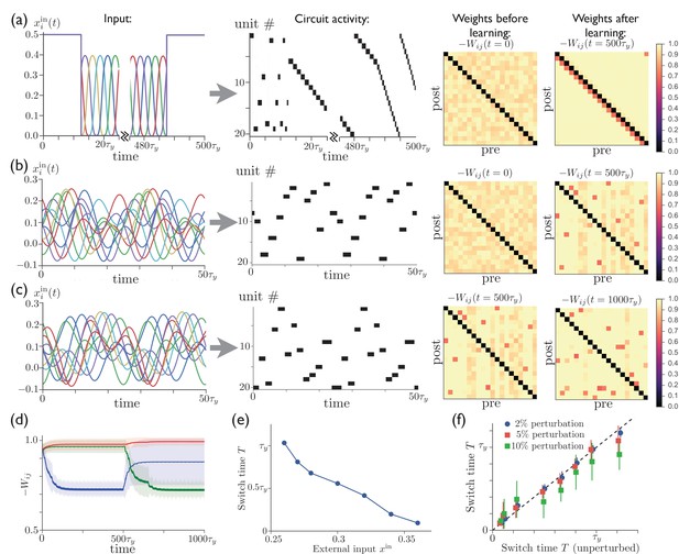
Repeated external input can tutor striatum to produce sparse activity sequences.

(a) A regular sequence of pulse-like inputs (only 10 inputs are shown for clarity; $25 τ_{y}$ = 1 cycle) (left) leads to a sequential activity pattern (center) and, via anti-Hebbian plasticity, converts a random connectivity matrix (at $t = 0$ ) to a structured matrix after 20 cycles (at $t = 500 τ_{y}$ ) (right). The input during the first half of the first cycle and the last half of the last cycle has been replaced by constant input to all units, which leads to a short random sequence before training and to a long specific sequence following training, with the sequence speed determined by the level of tonic input. (b) Starting with random connectivity between units (at $t = 0$ ), each unit is driven with a distinct time-varying input consisting of a random superposition of sine waves (two cycles of which are shown for 10 inputs) which produces a repeating activity sequence. Anti-Hebbian learning results in a structured matrix after 20 cycles (at $t = 500 τ_{y}$ ). (c) 20 cycles with a new input elicits a different activity pattern and overwrites the prior connectivity to a new structured matrix (at $t = 1000 τ_{y}$ ). (d) The evolution of the synaptic weights during the learning in ‘b’ and ‘c’. The blue, green, and red lines show the average weights of synapses involved in the first pattern, the second pattern, and neither pattern, respectively. (The weights shown in blue are not all repotentiated in the second training period due to the fact that some of these synapses are from units that are not active in the second sequence. For these weights ${\bar{x}}_{j} \approx 0$ in Equation 2, and thus they do not learn.) (e) The average time for switching from one unit to the next as a function of the constant external input after learning. (f) The switch times are robust to random perturbations of the weights. Starting with the final weights in ‘c’, each weight is perturbed by $Δ W_{i j} = p ξ_{i j} ⟨ W_{i j} ⟩$ , where $ξ_{i j} \sim (0, 1)$ is a normal random variable, and $p = 0.02$ , 0.05, or 0.10. The perturbed switch times (slightly offset for visibility) are averaged over active units and realizations of the perturbation. Learning-related parameters are $τ_{w} = 3 τ$ , $α_{1} = 0.05 / τ$ , and $α_{2} = 0.02 / τ$ .

https://doi.org/10.7554/eLife.26084.005

Figure 5

Download asset Open asset

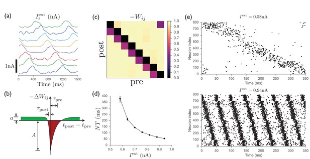
Spiking model of striatum.

(a) Input currents to each of 8 distinct clusters of 100 neurons each (offset for clarity). This input pattern causes sequential activation of the clusters and is repeated noisily several times while the recurrent weights are learned. (b) Schematic anti-Hebbian spike-timing-dependent plasticity (STDP) rule for recurrent inhibitory synapses, showing that synapses are depotentiated when pre- and post-synaptic spikes are coincident or sequential, and potentiated if they are not. (This STDP curve applies whenever there is a presynaptic spike; there is no weight change in the absence of a presynaptic spike; see Materials and methods for specific mathematical details.) (c) Average recurrent inhibitory weights between clusters in a spiking network after learning with STDP. (d) After the weights have been learned, driving the network with tonic inputs of varying amplitudes leads to a rescaling of the period of the activity pattern. (e) Two examples of the time-rescaled activity patterns in the trained network with different values of tonic input current.

https://doi.org/10.7554/eLife.26084.006

Figure 6

Download asset Open asset

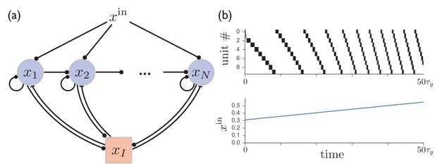
A network of excitatory units with shared inhibition exhibits variable-speed sequences.

(a) A network of $N$ excitatory units are connected by self-excitation, feedforward excitation, and shared inhibition. (b) Just as in the recurrent inhibitory network, this network exhibits sparse sequential firing when the excitatory synapses are made depressing, with the speed of the sequence controlled by the level of external input. Parameters are $β = 0.2, τ_{y} = 20 τ, τ_{I} = τ, J^{E I} = J^{I E} = 1, J_{i j} = 0.6 δ_{i j} + 0.2 δ_{j + 1, j}$ .

https://doi.org/10.7554/eLife.26084.007

Appendix 1—figure 1

Download asset Open asset

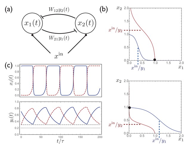
A simple circuit with two units exhibits activity switching.

(a) A simple two-unit network with activities $x_{1} (t)$ and $x_{2} (t)$ , symmetric inhibitory connectivity, and constant input $x^{in}$ . (b) Curves along which, for given fixed values of $y_{j}$ , the time derivatives ${\dot{x}}_{1, 2} = 0$ , with the intersection of these curves describing a stable fixed point. Depending on the relative values of $y_{1}$ and $y_{2}$ , the fixed point occurs at either $(x_{1}, x_{2}) \approx (1, 0)$ (top) or $(x_{1}, x_{2}) \approx (0, 1)$ (bottom). (c) When $y_{j} (t)$ are included as dynamical variables, the synaptic depression leads to periodic switching between the two stable solutions.

https://doi.org/10.7554/eLife.26084.008

Appendix 2—figure 1

Download asset Open asset

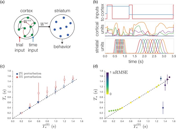
A trained recurrent network exhibits sequences that are less robust and less able to generalize.

(a) Schematic of the model. The cortical units receive trial-specific inputs and project to striatum. Striatal units are not recurrently connected. The corticocortical and corticostriatal weights $W^{cc}$ and $W^{sc}$ are set as per the text. (b) Model simulation. Upper: Inputs to model. Red trace marks initiation of trials; blue trace indicates the target time for the trial. Middle: Sample cortical units. Lower: Striatal units. (c) Means and standard deviations of best-match times as a function of target times with random weight perturbations of 2 or 5%. Open symbols denote target times for which the nRMSE exceeded 0.3 on greater than 25% of trials. (d) Best-match times for a model trained on time intervals ranging from 0.4 s to 1.2 s, and then tested from 0.1 s to 1.5 s. The colors indicate the means of the nRMSEs of the trials at each target time.

https://doi.org/10.7554/eLife.26084.009

Download links

A two-part list of links to download the article, or parts of the article, in various formats.

Downloads (link to download the article as PDF)

Article PDF

Open citations (links to open the citations from this article in various online reference manager services)

Mendeley

Cite this article (links to download the citations from this article in formats compatible with various reference manager tools)

James M Murray
G Sean Escola

(2017)

Learning multiple variable-speed sequences in striatum via cortical tutoring

eLife 6:e26084.

https://doi.org/10.7554/eLife.26084

Sign up for email alerts

Privacy notice