Dipolar extracellular potentials generated by axonal projections
- Humboldt-Universität zu Berlin, Germany
- University of Maryland, United States
- Bernstein Center for Computational Neuroscience, Germany
- RWTH Aachen, Germany
- Einstein Center for Neurosciences, Germany
Figures
Figure 1
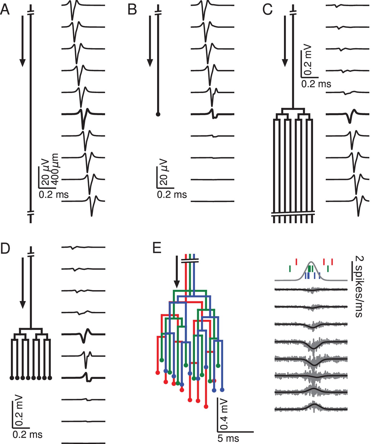
Relationship between axon morphology and extracellular potential.
Multi-compartment simulations of action potentials traveling along axons with varying morphologies, as indicated by the diagram on the left-hand side of each subfigure. Action potential propagation direction indicated by arrow. Waveforms, shown on the right-hand side of each subfigure, were recorded at a horizontal distance of 150 µm from the axons. The vertical depth is indicated by the plot position, spaced by 400 µm. Horizontal plot location and distances between axons are for illustration only, all axons were simulated to lie on a straight line. (A) Action potential in a quasi-infinitely long, straight axon. (B) Terminating axon. Action potential waveform closest to the termination thickened for emphasis. (C) Branching axon. The axon branches multiple times within of 200 µm. Thicker waveform at the center of the bifurcation zone. (D) Combined bifurcations and terminations. Note the larger voltage scales in C and D, which correspond to the different number of fibers. (E) Response in a population of 100 randomized morphologies, three of which are shown schematically (colored). Activity consists of spontaneous background activity (100 spikes/s) superimposed with a brief Gaussian pulse of heightened spike rate (2000 spikes/s). Spike rate and example spike times for the three morphologies are shown at the top. Right: gray lines show activity of full population averaged over 40 trials, while the black lines show the low-pass (<1 kHz) component. Note that the time and voltage scales are different from A-D. In all graphs, spatial scales are the same, as indicated by the scale bar in A.
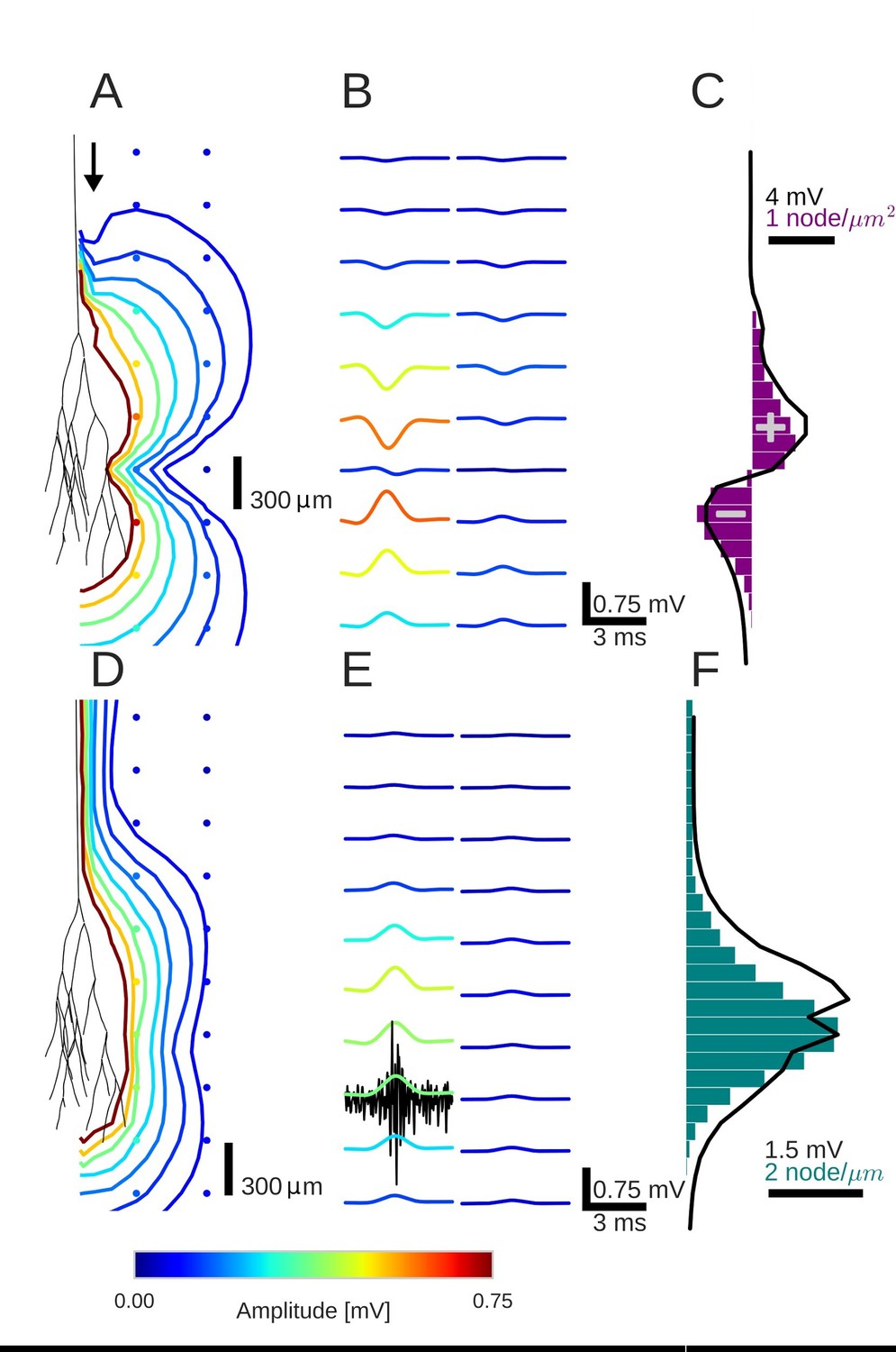
Figure 2
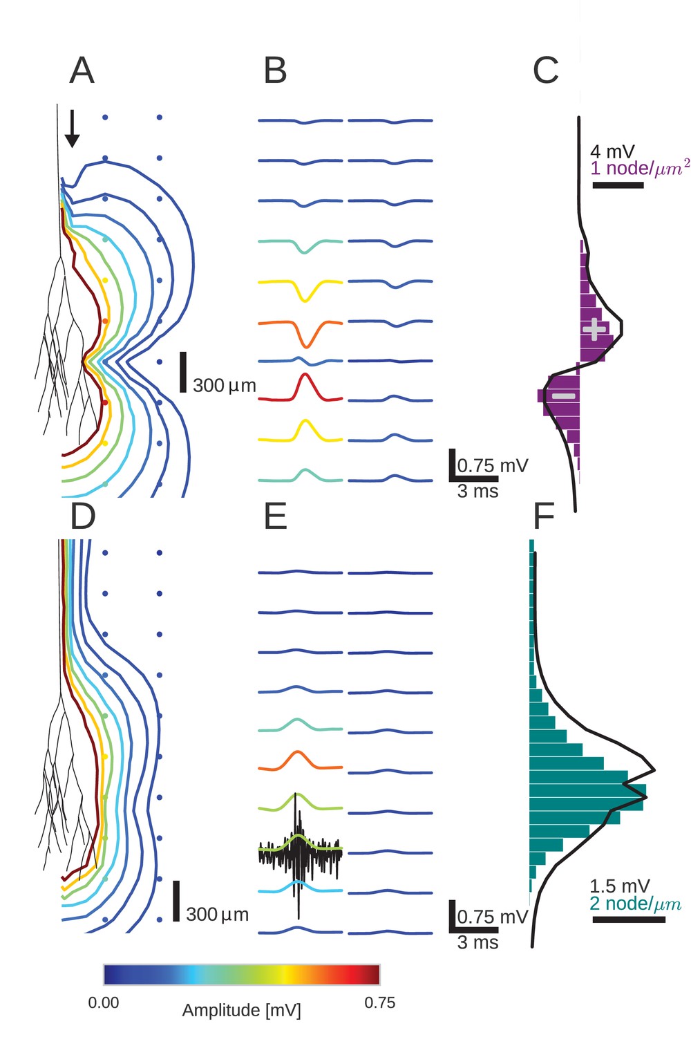
An activity pulse in an axonal projection generates a dipole-like extracellular field potential (EFP).
(A) Modeled example axon from the simulated bundle in black, along with iso-potential lines for the low-pass filtered (<1 kHz) EFP signature of the activity pulse. The contours (amplitudes in mV as indicated by colorbar) show the typical double-lobe of a dipole. (B) The low-pass filtered EFP waveforms, recorded at the locations of the colored dots in A, show mostly unimodal peaks. The peak amplitude reverses polarity as a function of recording location in the vertical direction. The reversal occurs by inverting the amplitude with approximately unchanged shape. (C) Progression of the maximum low-pass filtered EFP amplitude with depth (black line) at a distance of 100 µm from the trunk (indicated by arrow in A). The amplitude closely follows the local change (spatial derivative) in number of nodes per unit length (purple histogram), which is proportional to the difference in number between bifurcations and terminations. (D) Modeled axon from bundle as in A, and iso-potential contours for the multi-unit activity (MUA) component. (E) Response waveforms of the MUA component. High-pass filtered (>2.5 kHz) component (the first processing stage for calculation of MUA, see Materials and methods) in black. (F) Maximum amplitude of the MUA component (black line) follows the number of fibers (teal-colored histogram). Note the different units of the histograms in (C) and (F), due to the fact that (C) is the derivative in space of (F).
Figure 3
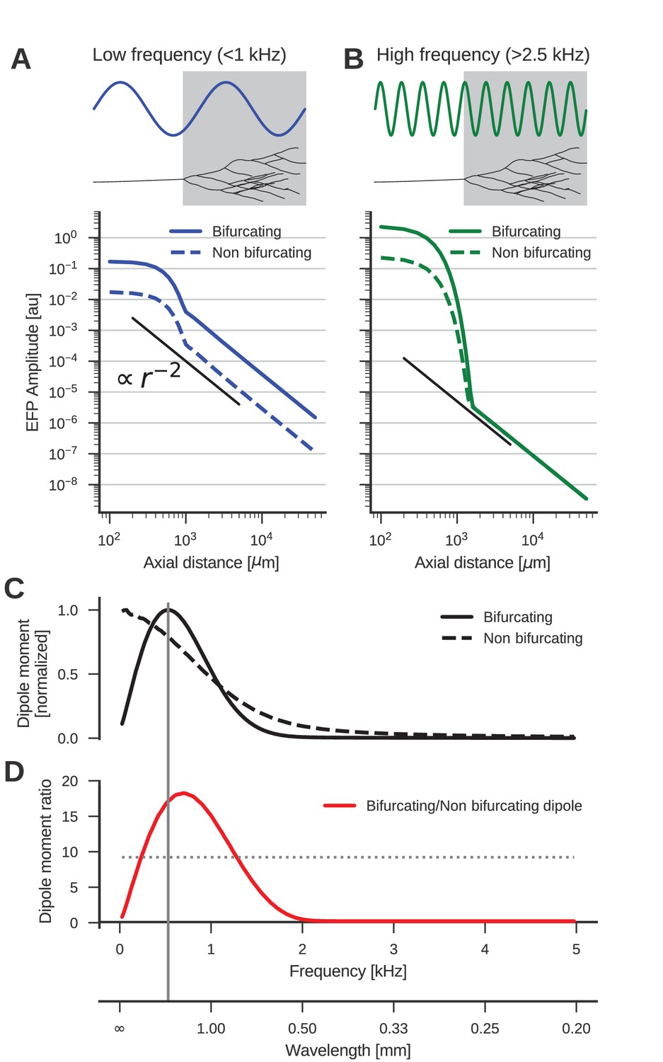
The low-frequency (<1 kHz) component of the axon bundle EFP is influenced supralinearly by a projection zone, while the high-frequency (>2.5 kHz) component is not.
(A) Scaling of the low-frequency (<1 kHz) EFP component. (Top) The spatial wavelength of the membrane potential oscillation (blue) is larger than the width of the projection zone (gray). (Bottom) The amplitude of the low-frequency EFP component for the bifurcating case (solid line) decays with with axial distance from the axon bundle. It always exceeds the EFP amplitude of the non-bifurcating case (dashed line). Note the double-logarithmic scale. Axial distances are calculated from the center of the terminal zone. For comparison, scaling that follows is indicated with the black line. (B) Same as A but for the high-frequency (>2.5 kHz) EFP component. (Top) The spatial wavelength of the membrane potential oscillation (green) is much smaller than the width of the projection zone (gray). (Bottom) The amplitude of the high-frequency EFP decays several orders of magnitude within the terminal zone, and the amplitude is larger in the bifurcating case (solid line) compared to the non-bifurcating case (dashed line). Far away from the terminal zone, i.e., for axial distances mm, they decay proportional to but with similar amplitudes. (C) Normalized dipole moments of the bifurcating and non-bifurcating bundles as a function of frequency. (D) Ratio of the dipole moments between bifurcating and non-bifurcating cases (red line), compared to the maximum ratio 10 of the number of fibers (dotted line), to indicate supralinear (>10) and sublinear (<10) contributions. Vertical gray line in C and D indicates the width (~2 mm) of the projection zone.
Figure 4
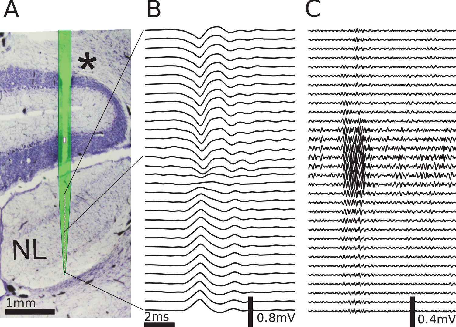
Multielectrode recordings in the barn owl show dipolar axonal EFPs.
(A) Photomicrograph of a 40 µm thick transverse Nissl stained section through the dorsal brainstem, containing a superimposed, to scale, diagram of the multielectrode probe. The probe produced a small slit in a cerebellar folium overlying the IVth ventricle (*), and penetrated into the nucleus laminaris (NL). The recordings were made in NL, and electrodes extended to both sides of the nucleus. The outline of the probe is shown in light green, with the recording electrodes indicated by magenta dots, and the reference electrode as a magenta rectangle. The low-frequency (<1 kHz) component (B) and the high-frequency (>2.5 kHz) component (C) are ordered in the same way as the electrodes, with three examples connected to their recording sites by black lines. The time scales in B and C are identical (indicated by scale bar). Traces were averaged over 10 repetitions. Voltage scales are indicated by individual scale bars.
Figure 5
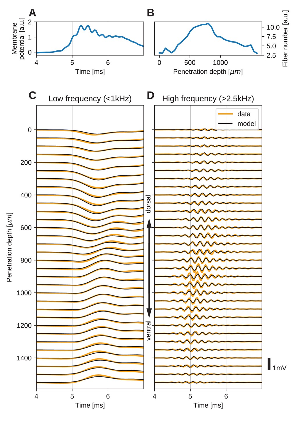
The spatial structure of EFPs recorded from the nucleus laminaris of the barn owl can be explained by a model of axonal field potentials (for details, see Materials and methods).
(A) Membrane voltage, averaged across fibers, in the model when fit to the data. (B) Fitted number of fibers in the model as a function of penetration depth. (C) Low-frequency ( kHz) components of the EFP in response to a click stimulus at time 0 ms, at different recording depths. The depth is measured in the direction from dorsal to ventral. Recorded responses (orange) are shown along with model fits (black). (D) High-frequency ( kHz) responses in recordings (orange) and model (black). Recorded traces were averaged over 10 repetitions.
Author response image 1
Author response image 2
Tables
Table 1
Parameter values used for the multi-compartment model which were modified from those used by Simon et al. (1999).
https://doi.org/10.7554/eLife.26106.007| Symbol | Meaning | Value | Value used by Simon et al. (1999) |
|---|---|---|---|
| axial resistance | 50 cm | 200 cm | |
| maximum sodium conductance | 2.4 S/cm2 | 0.32 S/cm2 | |
| maximum low-threshold potassium conductance | 0.1 S/cm2 | 3 mS/cm2 | |
| maximum high-threshold potassium conductance | 1.5 S/cm2 | 30 mS/cm2 | |
| leak conductance in node | 1 mS/cm2 | 0.28 mS/cm2 | |
| leak conductance in myelin | 1 S/cm2 | 35 S/cm2 | |
| leak reversal potential | −72 mV | −45 mV | |
| potassium reversal potential | −80 mV | −60 mV | |
| sodium reversal potential | 50 mV | 40 mV | |
| membrane capacitance in myelin | 1 nF/cm2 | 12 nF/cm2 |
Additional files
-
Transparent reporting form
- https://doi.org/10.7554/eLife.26106.008
Download links
A two-part list of links to download the article, or parts of the article, in various formats.
Downloads (link to download the article as PDF)
Open citations (links to open the citations from this article in various online reference manager services)
Cite this article (links to download the citations from this article in formats compatible with various reference manager tools)
Dipolar extracellular potentials generated by axonal projections
eLife 6:e26106.
https://doi.org/10.7554/eLife.26106


