Cerebellar re-encoding of self-generated head movements
Figures
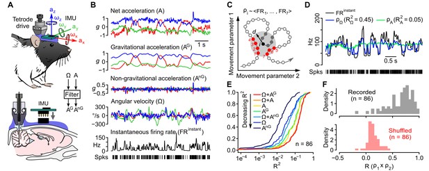
Caudal cerebellar units are sensitive to different combinations of rotational and gravitational information.
(A) Orientation of the inertial measurement unit (IMU) on the animal’s head and tetrode placement. An algorithm (‘filter’, see Appendix) was used to calculate the gravitational (AG) and non-gravitational (AnG) components of acceleration (A) using angular velocity (Ω) information. (B) Traces showing the instantaneous firing rate (FRinstant) of an example unit and inertial signals recorded simultaneously (A and Ω) or calculated offline (AG and AnG). (C) Principle of the model-free resampling method (see Appendix for details). Recordings of head movements can be described as sequences of points in a multidimensional parameter space (circles and line, here represented in a 2D space). At a given time point i (black circle), the estimated firing rate ρi is the mean of FRinstant values observed for neighboring points in the parameter space within a distance d (red circles) that did not occur immediately before or after i (filled gray circles). (D) Firing rate estimates calculated using Ω (ρΩ) or A (ρA) and FRinstant of an example unit. The values of the square of the Pearson correlation coefficient (R2) between FRinstant and firing rate estimates are indicated under parenthesis. (E) Cumulative distribution of R2 for firing rate estimates calculated using different combinations of inertial parameters (n = 86 units). (F) Distribution of Pearson correlation coefficients (R) between independent firing rate estimates, calculated using the combination of inertial parameters yielding the best estimate for each unit (gray histogram, mean R = 0.65 ± 0.23, n = 86 units). A null distribution was calculated using shuffled spike trains (red histogram, average from 10 iterations, mean R = 0.14 ± 0.10, n = 86 units, see Appendix).
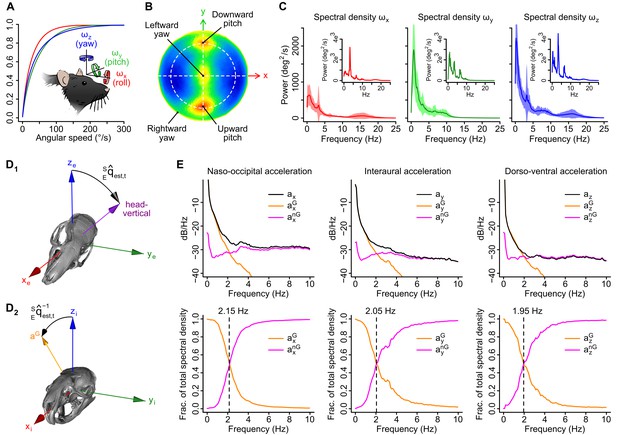
Head angular velocity and acceleration signals in freely moving rats.
(A) Average cumulative distributions of the three components of angular velocity in the sensor frame (n = 16 rats) and sketch depicting their orientation relative to the animal’s head. Arrows indicate rotation directions that produce positive angular velocity values. (B) Lambert azimuthal equal-area projection of the average spherical density distribution of angular velocity vector directions (n = 16 rats). The dashed circle represents the equator (coincident with the head’s horizontal plane). Most rotations are executed around the interaural axis (upward and downward pitch rotations) or around the head-vertical axis (leftward or rightward yaw rotations). (C) Average power spectral density (PSD) of angular velocity signals (n = 16 rats). Example PSDs for one recording are shown in the insets. (D1–2) Estimation of the orientation of gravity in the sensor frame. D1: The output of the orientation filter is a quaternion representation of a 3D rotation in the Earth frame (xe, ye, ze), noted , that brings the sensor from an initial orientation (here chosen as upright) to the current estimated orientation. D2: the orientation of the gravity vector (aG) in the sensor frame (xi, yi, zi) is obtained by applying the converse rotation (using the quaternion conjugate ) to the initial gravity vector (aligned with zi in the initial sensor orientation). (E) Top: average logarithmic PSD of raw acceleration (black) and its gravitational (orange) and non-gravitational (purple) components along the three axes of the sensor (n = 16 rats). Bottom: average fraction of the total spectral density of acceleration carried by the gravitational (orange) and non-gravitational (purple) components. Dashed lines indicate frequencies below which the spectral density is dominated by gravitational acceleration.
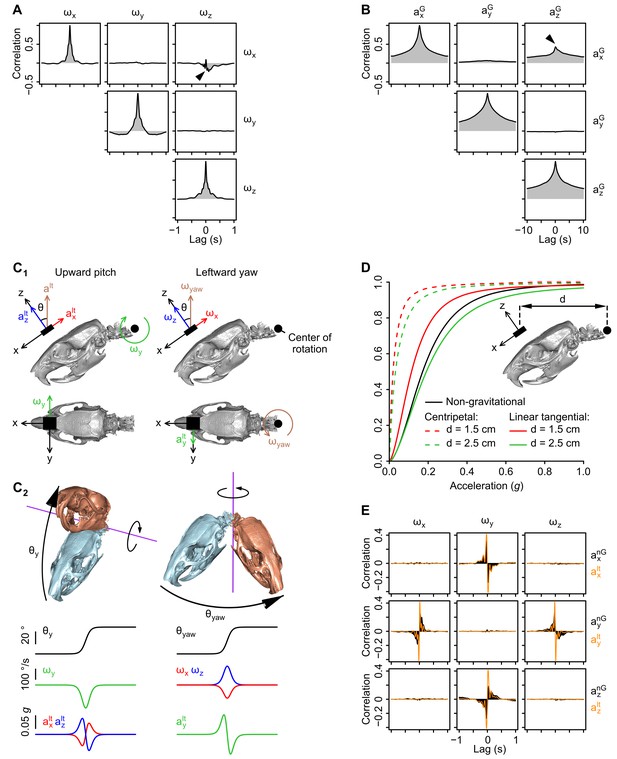
Geometrical and temporal coupling of head inertial signals during self-motion.
(A) Auto and cross-correlations of angular velocity signals (ωx, ωy, ωz; see axes orientation in Figure 1—figure supplement 1A). The anti-correlation between ωx and ωz (black arrowhead) can be explained by the fact that the head tends to be tilted (pitched down) during left-right (yaw) head rotations. (see panel C). (B) Auto and cross-correlations of gravitational acceleration signals (axG, ayG, azG; see axes orientation in Figure 1A). The positive correlation between axG and azG (black arrowhead) is due to the fact that both signals co-vary during pitch rotations (see panels C1 and C2). (C1-2) Calculation of linear tangential accelerations produced by pitch (up-down) and yaw (left-right) head rotations. C1: Side- and top-view of the head in its resting posture (tilted 35° nose down as shown in Blanks and Torigoe (1989)). Pitch and yaw rotations are executed around a point located in the animal’s neck (black circle), and thus produce a measurable linear tangential acceleration at the level of the sensor (black rectangle). An upward pitch rotation (left) produces negative ωy values and linear tangential accelerations along x and z of opposite signs (axlt and azlt). A leftward yaw rotation (right) produces negative ωx values and positive ωz values as well as a positive linear tangential acceleration along y (aylt). C2: Temporal profiles of angular velocity and linear tangential acceleration values for an upward pitch (left) and a leftward yaw (right) rotation. (D) Cumulative distribution of the average norm of centripetal (dashed color lines) and linear tangential (solid color lines) acceleration vectors resulting from pitch/yaw rotations, calculated for different distances (d) between the sensor and the center of rotation (n = 16 rats; see the Appendix for a detailed description of the calculation). The cumulative distribution of the average non-gravitational acceleration calculated using the orientation filter (see Figure 1—figure supplement 1D) is shown as a solid black line. The norm of linear tangential acceleration theoretically produced by pitch/yaw head rotations assuming d 2 cm (a realistic assumption) is comparable to the norm of non-gravitational acceleration calculated from the data. (E) Cross-correlation pattern between angular velocity (ωx, ωy, ωz) and non-gravitational acceleration (axnG, aynG, aznG), shown in black. The cross-correlation between angular velocity and the linear tangential acceleration theoretically resulting from head rotations (axlt, aylt, azlt, assuming that pitch and yaw rotations are executed as in C1) is superimposed in orange. Note that the two patterns of cross-correlation are similar.
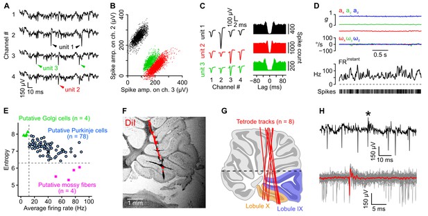
Isolation and classification of recorded units.
(A) Raw (unfiltered) electrophysiological signals from one tetrode in which three units were isolated. (B) Amplitude of sorted spikes on a pair of channels showing the three units visible in A. (C) Average unfiltered spike waveforms (left) and autocorrelograms (right) for the three units shown in A and B. The autocorrelograms were used to check the quality of the clustering (see Appendix). (D) Acceleration (ax, ay, az), angular velocity (ωx, ωy, ωz) and instantaneous firing rate (FRinstant) of one unit during a period of head immobility. In this example, the coefficient of variation of ISIs is 0.42. (E) Classification of recorded units based on the criteria established by Van Dijck et al., (2013) (see Appendix). Putative mossy fibers (n = 4, purple stars) were identified by their low entropy (cut-off set at 6.3) and putative Golgi cells (n = 4, green triangles) were identified based on their low firing rate (cut-off set at 12 Hz). Other units were classified as putative Purkinje cells (n = 78). (F) Representative tetrode track identified in the brightfield picture of a parasagittal slice. Tetrode were coated with DiI. A binarized epifluorescence image showing the DiI signal (red) was overlayed on the brightfield picture. (G) Tetrode tracks (red lines) reconstituted for eight rats after posthoc histological examination (as in F), superimposed on an atlas image of a parasagittal cerebellar slice. The most caudal lobules (lobules IX and X) are highlighted in colors. The horizontal black dashed line represents the upper limit of recordings. (H) Example unit in which complex spikes were detected. Top: unfiltered trace showing a single complex spike (asterisk). Bottom: averate complex spike waveform (in red), calculated from 25 traces (gray, overlaid). Note the characteristic pause in simple spike activity following the complex spike.
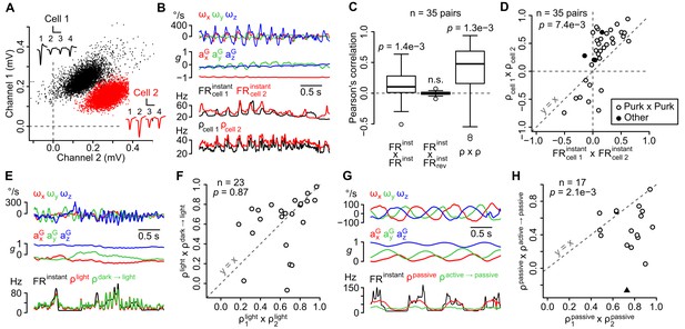
The sensitivity of recorded units is similar in the same recording site, does not depend on visual cues, but differs between active and passive movements.
(A) Amplitude of sorted spikes on a pair of channels and average spike waveforms of two neighboring units (scale bars: 0.3 mV and 1 ms for cell 1, 0.15 mV and 1 ms for cell 2). Channel numbers are indicated above the waveforms. (B) Example traces showing inertial parameters and the instantaneous and estimated firing rates of the two units shown in A. (C) Boxplots of Pearson correlation coefficients between instantaneous (FRinstant × FRinstant) or estimated (ρ × ρ) firing rates of neighboring units (n = 35 pairs). The correlation between FRinstant was lost if the firing rate of one unit was time-reversed (FRinstant × FRrevinstant, p=0.49; p-values above the boxplots were computed using a one-sample Wilcoxon test – null hypothesis: median = 0). (D) Graph comparing Pearson correlation coefficients between firing rate estimates (ρcell 1 × ρcell 2) and instantaneous firing rates (FRcell 1instant × FRcell 2instant) of neighboring units (p=0.0074, paired Wilcoxon test, n = 35 pairs). Pairs of putative Purkinje cells (n = 32) are shown in white. The diagonal dashed line represents the identity line. (E) Example traces showing inertial parameters and FRinstant for one example unit recorded in the light block. Color traces are firing rate estimates for the same recording calculated using data from the same block (ρlight) or from the dark block (ρdark light). (F) Graph comparing Pearson correlation coefficients between independent firing rate estimates in the light block (ρ1light × ρ2light) and between estimates of the firing rate in the light block calculated using data from either the light or dark block (ρlight × ρdark light). The p-value was computed using a paired Wilcoxon test. All units corresponded to putative Purkinje cells (n = 23). The diagonal dashed line represents the identity line. (G) Example traces showing inertial parameters and FRinstant for one example unit recorded in the passive block. Color traces are firing rate estimates for the same recording calculated using data from the same block (ρpassive) or from the passive block (ρactive passive). (H) Graph comparing Pearson correlation coefficients between independent firing rate estimates in the passive block (ρ1passive × ρ2passive) and between estimates of the firing rate in the passive block calculated using data from either the passive or active block (ρpassive × ρactive passive). The p-value was computed using a paired Wilcoxon test. All units corresponded to putative Purkinje cells, except one classified as a putative Golgi cell (black triangle, n = 17 units in total). The diagonal dashed line represents the identity line.
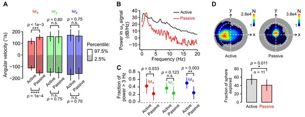
Statistics of head kinematics during active and passive movements.
(A) Average 2.5% (stripped bars) and 97.5% (plain bars) percentiles of angular velocity calculated from recording blocks during which movements were active (self-generated) or passive (generated by the experimenter, see Materials and methods; n = 11 recordings in both conditions). Vertical lines at the extremities of the bars represent the SD. Percentile values from each gyroscope axis (ωx, ωy and ωz in red, green and blue, respectively) were compared for the active and passive condition. Only roll velocity (ωx) percentiles differed between the two conditions (p=8.5 × 10⁻⁵ and p=7.7 × 10⁻⁴ for the 2.5% and 97.5% ωx percentiles respetively, Wilcoxon test). This corresponds to the fact that animals do not perform vigorous roll rotations in the freely moving conditions. (B) Representative power spectral density (PSD) distribution of the pitch angular velocity signal (ωy) acquired in an active (black) and in a passive (red) recording block. (C) Average (±SD) fraction of power distributed above 3 Hz for the signals acquired by each gyroscope axis (ωx, ωy and ωz in red, green and blue, respectively) in the active vs. passive condition (n = 11 recordings for both conditions). (D) Comparison of the span of head orientations relative to gravity (head tilt) in the active vs. passive condition. Top: representative examples of Lambert azimuthal equal-area projections of the spherical density distribution of the orientation of the gravity vector aG (expressed in the sensor’s reference frame) in the active (left) vs. passive (right) condition. The number of points N in the recording for each specific aG orientation is color-coded. The dashed white line represents the equator. The North pole is at the center. Bottom: average (±SD) percentage of the surface of the sphere that was explored by aG in both conditions (n = 11 recordings for both conditions).
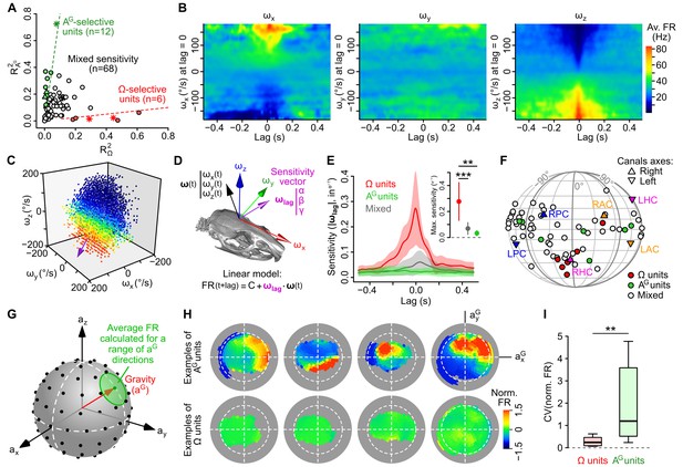
Subsets of caudal cerebellar units display preferential sensitivity to either head angular velocity or head tilt.
(A) Comparison of R2 values calculated based on gravitational acceleration (R2AG) or angular velocity (R2Ω) for all 86 units. Dashed lines delineate units with an R2 at least eight times greater for one parameter than the other and greater than 0.1 for the preferred parameter. Putative Purkinje cells, Golgi cells and mossy fibers are represented by empty circles, filled triangles and stars, respectively. (B) Inertio-temporal receptive fields of one example Ω-unit. (C) Firing rate (color-coded) of one Ω-unit (same as B) plotted as a function of the three components of angular velocity (see also Video 1) at the optimal lag. The colorbar is the same as in B. The unit’s optimal sensitivity vector at optimal lag (calculated using a linear regression, see D) is represented in purple (arbitrary scale). (D) Linear model used to characterize the units’ rotational tuning. For a given lag, the model assumes a linear tuning of firing rate to a preferred sensitivity vector ωlag. (E) Average (±SD) rotational sensitivity (norm of ωlag) plotted vs. lag values for Ω-units (n = 6), AG-units (n = 7) and other (‘mixed’) units (n = 53). Note that AG-units exhibit very weak rotational sensitivity. Only units with significant sensitivity were included (see Appendix). Inset: average (±SD) sensitivity of Ω-, AG- and mixed units at their optimal lag. **p=1.2 × 10⁻³, ***p=2.2 × 10⁻⁴. (F) Direction of optimal sensitivity vectors of Ω-units, AG-units and mixed units plotted on a pseudocylindrical projection. Triangles point up (resp. down) represent the excitatory direction of rotation of right (resp. left) semi-circular canals. LPC/RPC: left/right posterior canals; LHC/RHC: left/right horizontal canals; LAC/RAC: left/right anterior canals. (G) Calculation of tilt-dependent rate maps (see Appendix). The average firing rate was calculated for directions of the gravity vector (aG, in head coordinates) falling within 20° (green circle) of a series of points evenly distributed over a sphere (black dots). (H) Lambert azimuthal equal-area projections of spherical tilt-dependent rate maps for four example AG-units (top) and four example Ω-units (bottom). Dashed circles represent the equator (90° head tilt). (I) Boxplot of the CV of firing rate values in tilt-dependent rate maps for Ω-units (n = 6) and AG-units (n = 12). **p=0.0047.
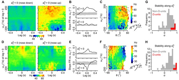
Tilt-dependence of rotational sensitivity in units with mixed gravitational and rotational sensitivity.
(A–F) Example units exhibiting a pitch tilt-dependent modulation of their apparent sensitivity to yaw velocity (ωz, measured in the sensor’s frame). In one unit (A–C), ωz sensitivity is visible for nose up orientations only (axG > 0). In the other unit (D–F), ωz sensitivity reverses for nose up vs. nose down orientations (axG > 0 vs. axG < 0). (A, D) Inertio-temporal receptive fields for ωz for nose up vs. nose down orientations. (B, E) Slope of the firing rate vs. ωz linear regression (calculated from the receptive fields in A and D), computed for different lag values in the nose up and nose down orientations. Shaded area represent the mean slope ±2 × SD calculated using shuffled spike trains (100 iterations). (C, F) Histogram showing the average firing rate (color coded) as a function of ωz and of the head’s pitch angle (θ). (G–H) Histograms of the stability index calculated for positive vs. negative values of axG (G) and for positive vs. negative values of ayG (H). The stability index was used to quantify the influence of head tilt on the direction of rotational sensitivity over a given lag range (see Appendix). Values close to 1 (resp. –1) denote a weak (resp. strong) influence of head tilt on the direction of rotational sensitivity. Histograms for non-Ω-units with significant rotational sensitivity (n = 60 units) are colored in gray and histograms for Ω-units (n = 6 units) are colored in red.
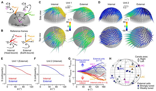
Different caudal cerebellar units encode head rotations in a head-bound or earth-bound reference frame.
(A) Method used to examine the influence of head tilt on rotational sensitivity. Optimal sensitivity vectors (ωopt) were calculated for different orientations of the gravity vector (aG) in head coordinates (: angular distance between different aG orientations). Collinearity (S) was assessed by computing the dot product of normalized sensitivity vectors. (B) ωopt vectors were calculated using internal (head-bound) or external (earth-bound) angular velocity values (see Appendix). ε: angle of elevation of ωopt vectors relative to the (x,y) plane of the reference frame in which they were calculated. (C–D) ωopt vectors of two examples units, calculated using internal (left) or external (right) angular velocity, positioned at locations corresponding to orientations of aG (in head coordinates) for which they were calculated, and color-coded according to their angle of elevation . (E–F) Collinearity of externally- (blue curve) and internally-referenced (red curve) sensitivity vectors vs. angular distance for the two units shown in C and D. (G) Difference between external and internal collinearity curves (S) for all units with significant rotational sensitivity (n = 66). Units with a strong external or internal tuning (ΔS > 0.5 or ΔS < −0.5 for in the 80–100° range) are highlighted in blue (n = 7) and red (n = 5), respectively. The two units shown in C and D are highlighted in purple (unit 1, shown in C) and orange (unit 2, shown in D). (H) Direction of external sensitivity vectors for the seven units highlighted in blue in G (dark blue circles), and for 12 units with a weaker external tuning (ΔS > 0.1 for in the 80–100° range, light blue circles), plotted on a pseudocylindrical projection. The excitatory direction of rotation of semi-circular canals is indicated as in Figure 3F.
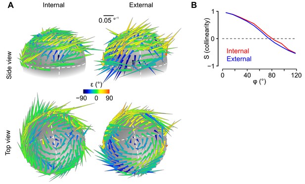
Rotational sensitivity map of a unit exhibiting no preferential tuning in an internal or external reference frame.
(A) 3D representation of rotational sensitivity vectors (see the legend of Figure 4C,D and the Appendix for details) of an example unit whose tuning does not seem to be better explained by an external or internal coding scheme. (B) Collinearity profile (see the Appendix for details) of the unit shown in A.

The model-free resampling approach is better at predicting firing rate than a ‘global’ linear model and is equivalent to a series of ‘local’ linear models calculated for different head tilts.
(A) Firing rate predictability computed by the model-free resampling approach (see Figure 1D–F and Appendix) using angular velocity and gravitational acceleration (R2Ω+ AG), plotted vs. the coefficient of determination (r2) of a ‘global’ linear model describing the firing rate as a combination of angular velocity, angular acceleration, and gravitational acceleration (p=1 × 10⁻¹³, paired Wilcoxon test, see Appendix and Figure 6—figure supplement 1). Each point represents one unit (n = 86 units). (B) Firing rate predictability computed by the model-free resampling approach using angular velocity and gravitational acceleration (R2Ω+ AG), plotted vs. the coefficient of determination of ‘local’ linear models describing the firing rate as a function of angular velocity and calculated for specific head tilts (p=0.24, paired Wilcoxon test). Each point represents one unit (n = 86 units). The arrowheads on the grey sphere symbolize ‘local’ optimal rotational sensitivity vectors (ωopt) calculated for specific orientations of the gravity vector in the sensor frame (see Figure 5A and Appendix).
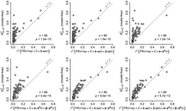
Performance of the model-free resampling approach vs. global linear models.
Firing rate predictability, computed by the model-free resampling approach (see Figure 1D–F and Appendix) using angular velocity and gravitational acceleration (R2Ω+ AG), was plotted vs. the coefficient of determination (r2) of ‘global’ linear models describing the firing rate as a combination of inertial parameters (see Appendix). The formula of each linear model is indicated in the label of the abscissa, where , , and are vectors representing the instantaneous angular velocity, angular acceleration, gravitational acceleration and jerk (time derivative) of the gravitational acceleration, respectively, and λ, ξ, α and β are vectors representing the corresponding coefficients of the fit. Each point represents one unit (n = 86 units). Note that the model-free approach based on angular velocity and gravitational acceleration always explains significantly more firing rate variance that global linear models (p-values calculated using paired Wilcoxon tests; see also Figure 6A).
Videos
Changes of orientation of the gravitational acceleration vector (aG) in the head reference frame during natural head movements.
This movie illustrates how gravitational acceleration information can be used to track head orientation relative to gravity (head tilt). Left: 3D view of a rat skull animated using a sequence of head rotations acquired from a freely moving rat. The head was positioned in 3D using the output of the orientation filter. Because the filter only outputs head tilt information, and not absolute orientation (comprising azimuthal information), the naso-occipital (x) axis of the head was maintained aligned in the same vertical plane. aG is represented by a purple arrow. Right: trajectory of aG (purple arrow) corresponding to the same movements and represented in the head reference frame. Because aG has a constant norm (of 1 g), its trajectory is contained within a sphere (represented in gray).
3D plot of the sensitivity of one example Ω-unit to head angular velocity (see Appendix).
The unit is the same as the one shown in Figure 3F. The average firing rate is color coded. The optimal rotational sensitivity vector ωopt calculated using a linear regression (see Appendix) is shown in purple (arbitrary scale) to show its alignment with the gradient of firing rate values.
Examples of 3D tilt-dependent rotational sensitivity maps.
This movie shows the 3D tilt-dependent rotational sensitivity maps of the three example units shown in Figure 4J. To generate these plots, rotational sensitivity vectors were calculated (using either internal or external angular velocity values) for different head tilts (as explained in the Appendix) and plotted as arrowhead.
Opposite changes of azimuth induced by the same pitch rotation (as measured by semi-circular canals) for two different head tilts.
This movie illustrates how internally-referenced angular velocity signals do not necessarily map to externally-referenced angular velocity signals. Here, two identical pitch rotation sequences (as measured by the semi-circular canals) are executed from two different situations, in which the head is tilted either to the right or to the left. When the head is tilted right, an upward pitch rotation induces a change of azimuth (head angular direction in the earth-horizontal plane, represented in gray) toward the right; but when the head is tilted left, the same pitch rotation induces a change of azimuth in the opposite direction.


