The liquid structure of elastin
Figures
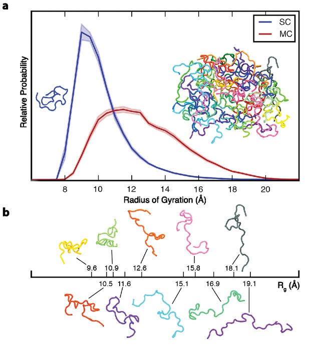
Ensemble-averaged polypeptide chain dimensions.
(a) Probability distribution of the radius of gyration, Rg, for SC (blue) and MC (red). Insets show representative backbone conformations of peptide monomer (left) and aggregate (right). (b) Aggregated chains are colored individually and ten of them are also shown below with their corresponding Rg to illustrate the conformational heterogeneity. In all figures, error bars indicate standard error. All the results reported in this and subsequent figures were obtained at 298 K unless otherwise noted.
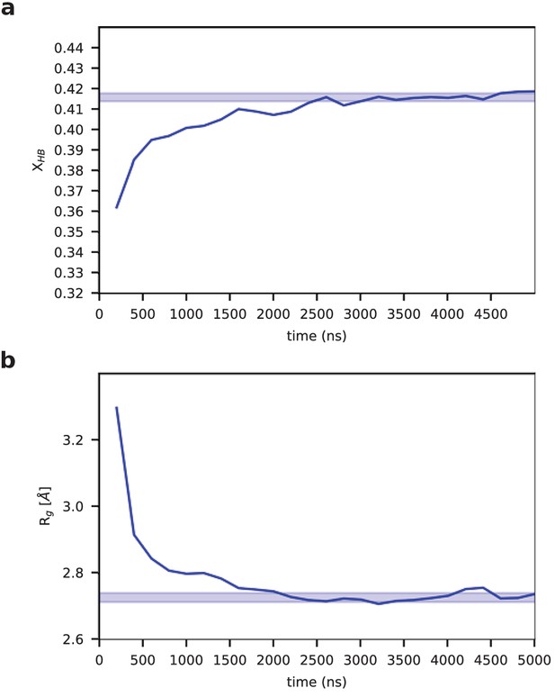
Formation and collapse of the aggregate.
Running averages of (a) the number of hydrogen bonds per residue, XHB, and (b) the radius of gyration, Rg.

Ensemble-averaged polypeptide chain dimensions with the TIP4P-D water model.
Probability distribution of the radius of gyration, Rg, for SC (blue) and MC (red) systems obtained using the charmm-modified TIP3P water model (Jorgensen et al., 1983; MacKerell et al., 1998) (as in Figure 1a), and the SC system obtained using the TIP4P-D water model (Piana et al., 2015) (green).
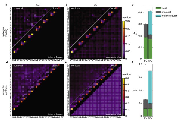
Peptide-peptide interactions.
Probabilistic description of hydrogen bonding (top row) and non-polar (bottom row) interactions of SC (a and d) and MC (b and e) systems. Panels (a), (b), (d) and (e) are contact maps for pairwise interactions between residues. The color of each square indicates the fraction of conformations in the ensemble for which that interaction is present. Nearest- and next-nearest-neighbour contacts are excluded for clarity in (d) and (e). Local interactions consist of sparse backbone hydrogen bonds and corresponding non-polar contacts. Non-local interactions consist primarily of non-specific non-polar contacts between side chains. With the absence of preferred non-local interactions, the statistical picture of the conformational ensembles is remarkably simple. Upon aggregation, local structure propensities are retained as non-local hydrophobic contacts become intermolecular contacts (below the diagonal in e). (c) Average number of chain-chain hydrogen bonds per residue, XHB. (f) Average number of non-polar contacts per residue, XNP. Both XHB and XNP are the sum of intramolecular (local and non-local) and intermolecular contributions. Details of the structural analysis methods are provided in Materials and methods and Supplementary file 1, Table S2.
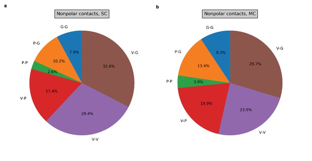
Non-polar contacts between residue pairs.
The fraction of non-polar contacts between each of the six possible residue pair combinations (V-G, V-V, V-P, P-P, P-G, G-G) is shown for the single chain (a) and multi-chain (b) systems.
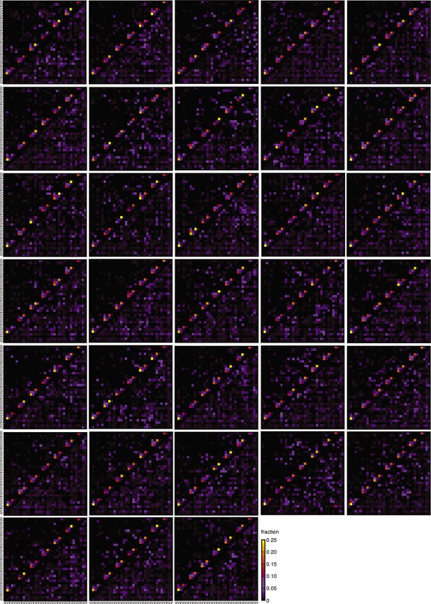
Hydrogen bonding contact maps.
A contact map is shown for each of the 33 independent MC simulations. The color scheme is the same as the one used in Figure 2.
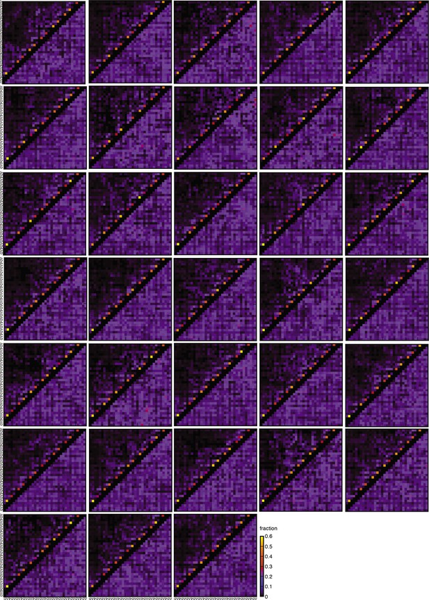
Non-polar contact maps.
A contact map is shown for each of the 33 independent MC simulations. The color scheme is the same as the one used in Figure 2.
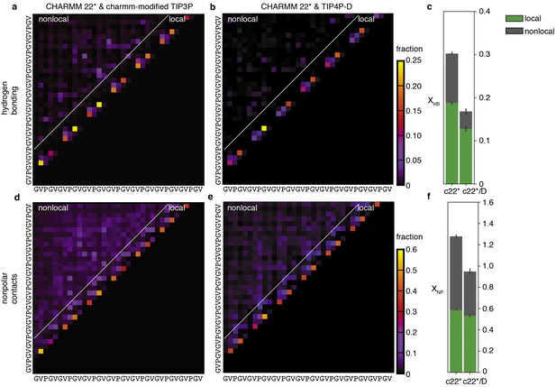
Peptide-peptide interactions for the SC ensemble obtained using the TIP4P-D water model.
Probabilistic description of hydrogen bonding and non-polar interactions of the SC system obtained using CHARMM 22* with the charmm-modified TIP3P water model (a and d; these results are the same as shown in Figure 2a,d) and CHARMM 22* with the TIP4P-D water model (Piana et al., 2015) (b and e). The color of each square in the contact maps indicates the fraction of conformations in the ensemble for which that interaction is present. (c) Average number of intrachain hydrogen bonds per residue for the ensemble obtained with CHARMM22* and charmm-modified TIP3P (c22*) and TIP4P-D (c22*/D). (f) Average number of non-polar contacts per residue. Both XHB and XNP are the sum of local and non-local contributions.
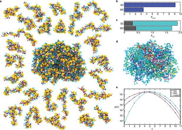
Peptide hydration in the liquid-like aggregate.
(a). Representative conformation of the aggregate with non-polar side chains (yellow), peptide backbone (oxygen, red; carbon, white; nitrogen, blue), and hydrogen-bonded water molecules (cyan). Peptide chains are shown individually on the periphery with bound water molecules. (b) Average number of water molecules in the hydration shell per residue, Xshell, for SC and MC systems (see Supplementary file 1, Table S2). (c) Average number of hydrogen bonds per residue, XHB. XHB is the sum of peptide-peptide hydrogen bonds (grey) and peptide-water hydrogen bonds (cyan), for both the SC and MC systems. (d) Same conformation as in panel a with bound water molecules shown as a transparent surface and peptides coloured individually. (e) Probability distribution, p(n), of water coordination number, n, for water molecules in the hydration shell of the SC (blue) and the MC (red) systems and in bulk water (cyan) at 298 K. Peptide-bound water molecules in the aggregate have fewer neighbors. The lines are shown to guide the eye.
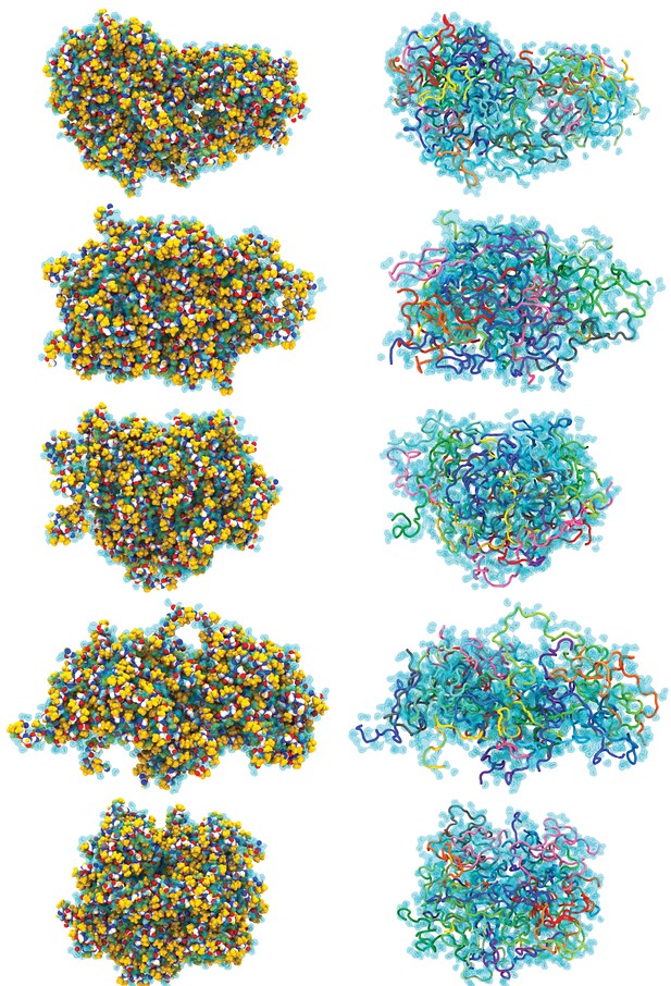
Conformations after 5 µs of simulation.
The final conformation of 5 of the independent simulations is shown in two representations. The color schemes are the same as in Figure 3a and d.
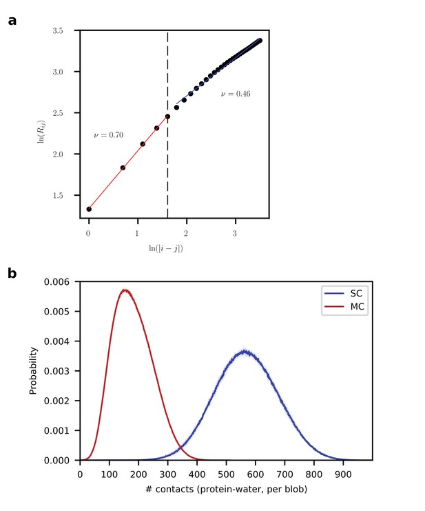
Hydration of blob-sized segments.
(a) The scaling of inter-residue distances is shown within a blob-sized segment of 5 residues (linear fit in red) and outside of a blob-sized segment (linear fit in blue). The scaling exponents differ in these two regimes, as expected based on the work of Tran and Pappu, 2006. (b) A histogram of the number of contacts between protein and water molecules per blob-sized segment is shown for both the SC and MC systems. Shading indicates standard error. Chain segments in the aggregate have, on average, far fewer contacts with water molecules, indicating that even the chains on the surface are significantly dehydrated compared to the chain in solution, which also has no water-excluding core.
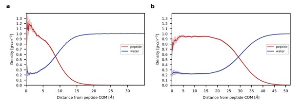
Radial density profiles.
(a). Density profiles for peptide (red) and water (blue) as a function of the distance from the center of mass (COM) of the peptide is shown for the single chain system. (b) Density profiles for peptide and water as a function of the distance from the COM of the aggregate is shown for the multi-chain system. Shading in (a) and (b) indicates standard error. Note that the large width of the transition region between the homogenous interior and bulk water reflects not only the higher hydration of residues at the surface but also the asphericity of the aggregate (see Figure 3—figure supplement 1).
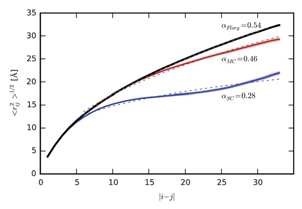
Intrachain distance scaling and comparison to the ideal, random-coil state.
Root-mean-square distance, <rij2>1/2, between residues i and j as a function of sequence separation, |i-j|, for SC (blue) and MC (red), and for the ideal, random coil state modeled using the SC simulations according to the method of Flory et al. (black) (Flory, 1969; Miller et al., 1967) described in detail in Supplementary file 1. Shading indicates standard error. In each case, the dotted line indicates the power law fit to the data, with the exponent α provided next to each curve.
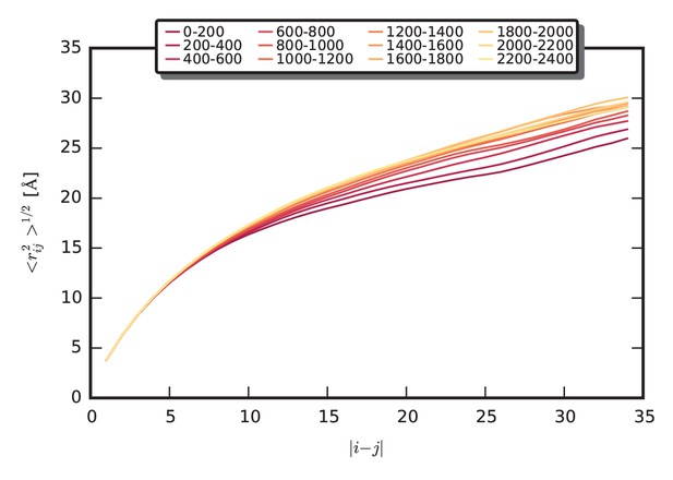
Equilibration of chain dimensions in the aggregate.
The mean separation distance is shown as a function of sequence separation for 200 ns time intervals of the simulation. The color scheme is given in the legend: each interval is colored from red to yellow, from the beginning to 2.5 µs. The initial expansion of the chains occurs in the first microsecond of the simulation, followed by a slight further collapse to the equilibrium dimensions.
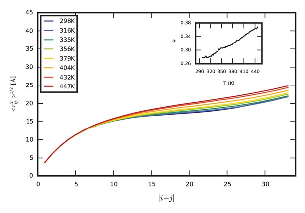
Temperature dependence of the conformational properties of the monomer.
The scaling of inter-residue distances (the same analysis as shown in Figure 5) is shown for the SC ensemble at a range of temperatures between 298 K and 447 K, covering the entire range of temperatures simulated. The chain undergoes a gradual, steady expansion as temperature with increasing temperature. The inset shows the fitted exponent α as a function of temperature. Extrapolating the linear increase in α vs. temperature, the chain would reach α = 0.5 (as expected for a random coil) at 664 K.
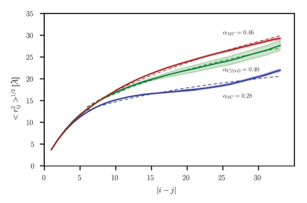
Intrachain distance scaling for the ensemble obtained using TIP4P-D.
Root-mean-square distance, <rij2>1/2, between residues i and j as a function of sequence separation, |i-j|, for the ensemble obtained using the CHARMM 22* force field with the TIP4P-D water model (green). Results for SC (blue) and MC (red) systems obtained using the CHARMM 22* force field with the charmm-modified TIP3P water model (as in Figure 5) are shown for comparison. Shading indicates standard error. In each case, the dotted line indicates the power law fit to the data, with the exponent α provided next to each curve.
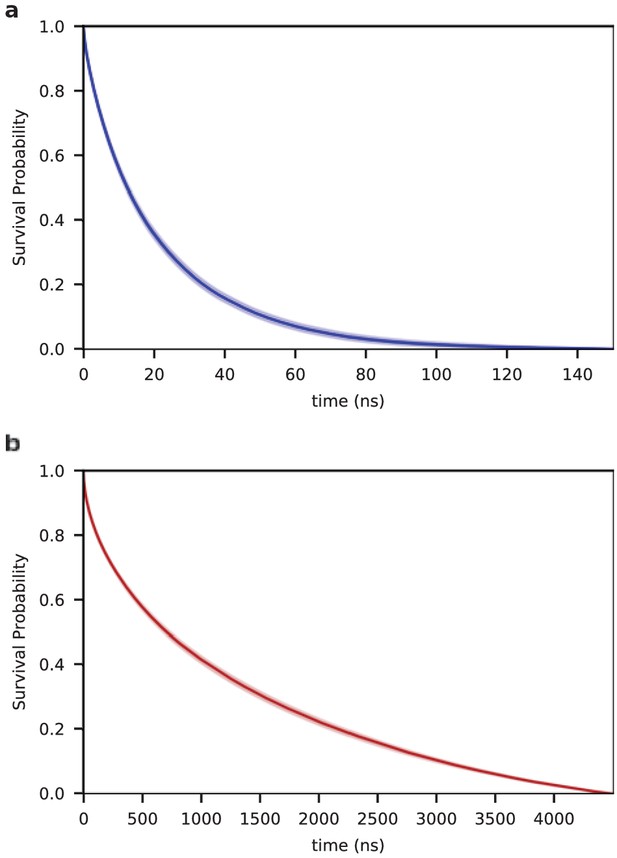
Kinetics of end-to-end contact formation.
Survival probability of the open state (without a contact between the chain ends) as a function of time for the single chain (SC) (a) and for the aggregated chains (MC) (b) . The lifetime of the open state is 21 ± 1 ns and 1140 ± 30 ns for the SC and MC systems, respectively.
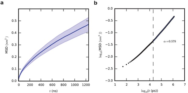
Chain dynamics within the aggregate.
(a) The mean squared displacement, MSD, of the central residue of the chain is shown as a function of time. This curve is an average over all chains (27 chains per system) and all simulations (33 in total), using only the second half of the trajectory in each case. Shading indicates standard error of the mean based on the 33 replicate simulations. (b) Anomalous diffusion is seen, and the exponent α is 0.578 (obtained by fitting the linear part of the curve for t > 20 ns).
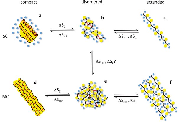
Structural basis of entropic elasticity in self-assembled elastomeric proteins.
Schematic description of polypeptide main chains (black), non-polar side chains (yellow), solvating water molecules (blue), and peptide-peptide hydrogen bonds (red) in monomeric (SC, top row) and aggregated (MC, bottom row) states. Globular proteins that unfold or misfold are prone to aggregation, which leads to highly ordered amyloid fibrils. Both the native (a) and amyloid (d) states of globular proteins are characterized by extensive secondary structure and a water-excluding hydrophobic core. Despite their hydrophobic character, elastin and other self-assembled elastomers cannot form such compact structures due to their high content in proline and glycine. Instead, they are hydrated and disordered both in their monomeric (b) and aggregated (e) states, so that they may readily undergo extension and elastic recoil (e-f). The role of the two dominant types of entropy, the hydrophobic effect (ΔSHP) and chain entropy (ΔSC), is highlighted. While the hydrophobic effect favors hydrophobic collapse (c→b, f→e), aggregation (b→e), and, if possible, compact, water-excluding states (b→a, e→d), conformational entropy favors disordered (b, e) over extended (c, f) and compact (a, d) states. As a result, both entropic effects contribute to elastic recoil. Adapted with permission from Rauscher et al. (2006), Structure (Rauscher et al., 2006).
Videos
In Video 1, the final 95 ns of a 5 microsecond trajectory of an aggregate is shown.
Each of the 27 peptide chains is colored individually. Frames in the movie correspond to conformations separated by 50 ps time intervals. A smoothing window of 2 frames was applied and all conformations were aligned to the first conformation for clarity using VMD (Humphrey et al., 1996). As can be seen in the movie, both the global structure of the entire aggregate as well as the conformation of individual chains within the aggregate fluctuate on the nanosecond timescale. Chains on the surface of the aggregate occasionally extend outward into the surrounding water (water molecules are not shown for clarity).
Tables
Populations and lifetimes of hydrogen-bonded turns.
https://doi.org/10.7554/eLife.26526.010| Turn | Population (%) | Lifetime (ns) | ||
|---|---|---|---|---|
| SC | MC | SC | MC | |
| VPGV* | 18 ± 1 | 16 ± 2 | 0.18 ± 0.02 | 0.19 ± 0.01 |
| VPGVG | 5.9 ± 0.9 | 4.6 ± 0.7 | 0.9 ± 0.3 | 0.8 ± 0.1 |
| PGV | 1.5 ± 0.1 | 2.0 ± 0.2 | 0.008 ± 0.002 | 0.009 ± 0.001 |
| PGVG | 2.3 ± 0.2 | 2.9 ± 0.3 | 0.30 ± 0.05 | 0.39 ± 0.03 |
| GVGV | 20 ± 3 | 17 ± 2 | 0.15 ± 0.02 | 0.24 ± 0.07 |
-
*A hydrogen-bonded turn refers to a hydrogen bond between the first and last residue in the sequences shown. For example, the VPGV turn has a hydrogen bond between valine 1 and valine 4.
Additional files
-
Supplementary file 1
Supplementary information: Supplementary Methods (Method to Compute the Average Dimensions of the Ideal, Random Coil State), Figure S1 and Tables S1 and S2.
- https://doi.org/10.7554/eLife.26526.023
-
Supplementary file 2
The supplementary file contains a coordinate file (prot_100ns.gro) and a trajectory file corresponding to the final 100 ns (4_9 ms_to_5 ms.xtc) of one of the aggregate simulations.
A larger trajectory file (4 ms_to_5 ms.xtc) corresponding to the final microsecond of the same simulation can be downloaded from the public repository figshare.com (S. Rauscher and R. Pomès, ‘Microsecond-long molecular dynamics trajectory of an aggregate of elastin-like peptides in water.’ DOI: 10.6084/m9.figshare.5532214).
- https://doi.org/10.7554/eLife.26526.024


