Model-based local density sharpening of cryo-EM maps
- European Molecular Biology Laboratory, Germany
- The Hamburg Centre for Ultrafast Imaging, Germany
Figures
Figure 1 with 1 supplement
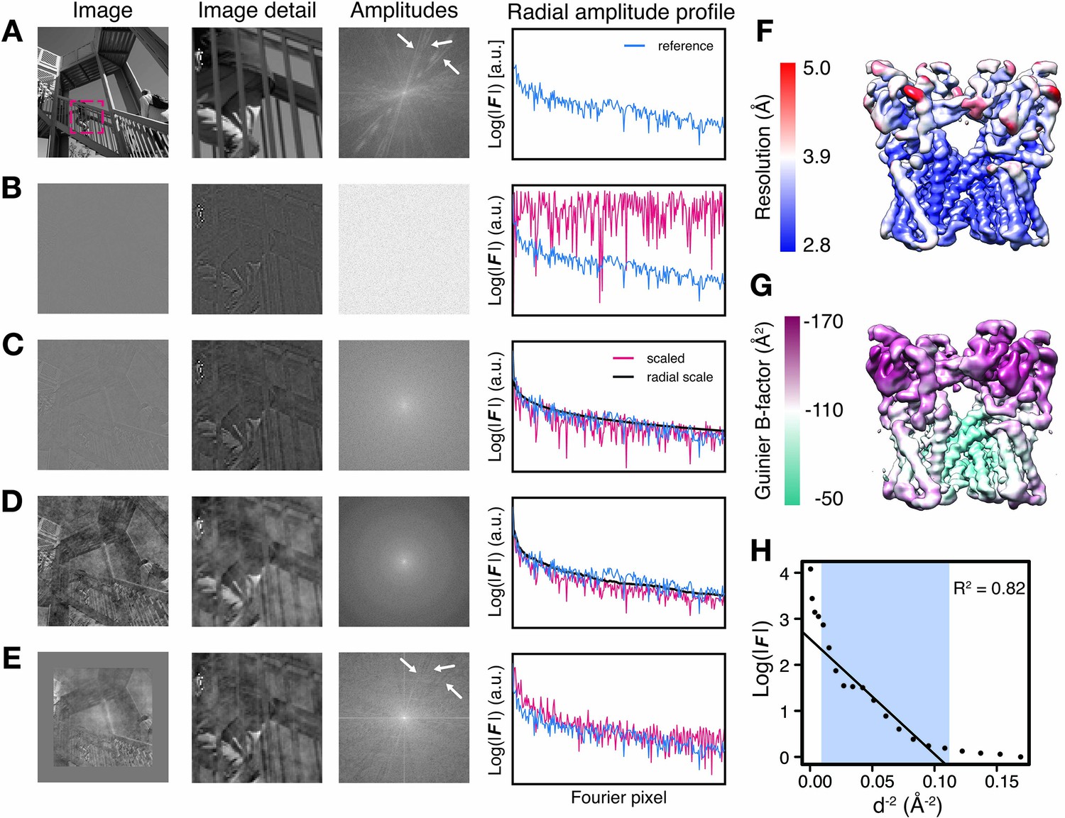
Illustration of local amplitude scaling (LocScale) using a 2D test image and determination local B-factors in cryo-EM maps.
(A) The original image (left), a magnified image detail (center left), the overall amplitude spectrum (center right) and the radially averaged amplitude profile (right) are displayed in panels along columns, respectively. Applied procedures are shown along rows. The radial amplitude profile of the reference, the scaled image and the applied scale are shown in blue, red and black, respectively. (B) Hybrid image resulting when amplitudes were replaced by random Gaussian noise and combined with phases from the original image in (A). The falloff of the amplitude profile of the hybrid image (red) is flat over the entire frequency range and hampers visual perception of image contrast. (C) Hybrid image from (B) when random amplitudes were scaled by a negative exponential estimated from the amplitude falloff of the original image. (D) Hybrid image from (C) with random amplitudes scaled by the average radial falloff profile from (A). (E) Hybrid image from (D) with amplitudes scaled locally to reference amplitudes from (A) computed in tiles of 128 × 128 pixel rolling windows. Note that diagonal lines in the amplitude spectrum (white arrows) arising from periodic image features are optimally recovered. Compare with the power spectrum of the original image. (F) Resolution estimates from local FSC calculation with a 24 Å sampling window mapped onto the surface representation of the TRPV1 channel (EMD-5778). (G) B-factors determined from local Guinier fitting in 24 Å sampling window mapped onto the surface representation of the TRPV1 channel (EMD-5778). (H) Guinier plot for a representative density window used for local B-factor estimation in (G). The linear falloff estimated from least squares fitting to the data is shown as straight line. The fitting interval ranging from 10 Å to the locally estimated resolution (here 3.1 Å) is highlighted in blue.
Figure 1—figure supplement 1
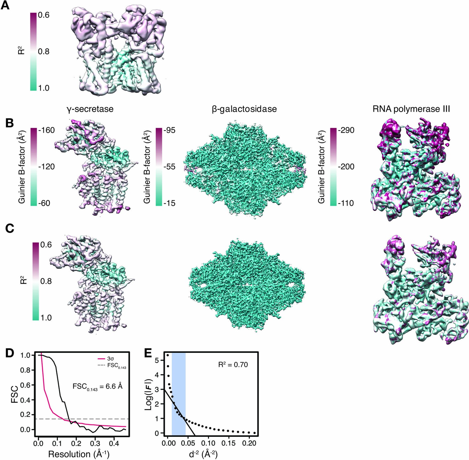
Local B-factor estimation by Guinier fitting.
(A) Coefficient of determination (R2) from local Guinier fitting mapped onto the molecular surface to TRPV1. (B) Distribution of B-factors estimated from local Guinier fitting mapped onto the molecular surfaces of γ-secretase, β-galactosidase and Pol III. (C) Coefficient of determination (R2) from local Guinier fitting as shown in (B) mapped onto the molecular surfaces of γ-secretase, β-galactosisdase and Pol III. (D) Local FSC curve shown for a representative 35 Å density window of Pol III. The estimated resolution is 6.6 Å based on FSC0.143 threshold and 3σ criterion. (E) Guinier plot of the density window in (D). The linear falloff estimated from least squares fitting to the data is shown as straight line. The fitting interval ranging from 10 Å to the locally estimated resolution (here 6.6 Å) is highlighted in blue.
Figure 2 with 2 supplements
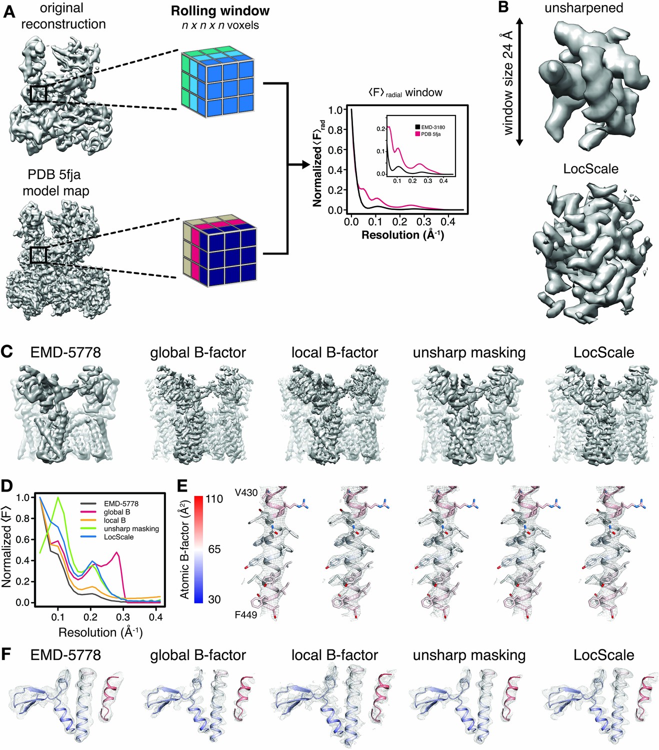
Generation of 3D LocScale density maps and comparison of global and local sharpening procedures.
(A) Schematic illustration of the LocScale procedure for a Pol III density map. Two equivalent map segments (rolling windows) are extracted from the original 3D reconstruction of EMD-3180 (top) and a map simulated from the atomic model (PDB ID 5fja) (bottom). For each rolling window, the radially averaged structure factor profile is computed and used to scale the amplitudes of the corresponding window of the original reconstruction. Note, the fine structure of the model amplitudes has a characteristic profile in the resolution range <10 Å due to protein secondary structure and deviates from a simple exponential falloff (inset). (B) Effect of amplitude scaling illustrated for an exemplary density window. The density contained within a window cube is shown before (unsharpened) and after (LocScale) application of amplitude scaling. The central voxel of the rolling window is assigned the map value after amplitude scaling. The procedure is repeated by moving the window along the map until each voxel has been assigned a density value based on the locally estimated contrast. (C) Side views of TRPV1 densities obtained with different sharpening methods. Far left, EMD-5778 unsharpened; left, global Guinier B-factor −100 Å2; middle, local Guinier B-factor; right, unsharp masking and far right, LocScale sharpening. (D) Radial amplitude profiles of the respective maps shown in (C). (E) Mesh representation of the densities for transmembrane residues 430–449 superposed on the atomic model (color-coded by atomic B-factor). The order from left to right is the same as in (C) and (F). Side chains are shown in stick representation. (F) Mesh representation for a peripheral density region superposed on the atomic model shown in ribbon representation and color-coded by atomic B-factor. B-factor scale as in (E).
Figure 2—figure supplement 1
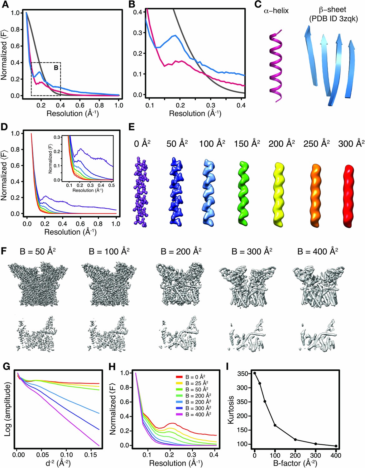
Effect of secondary structure and atomic B-factors on the radial structure factor amplitude profile.
(A) Typical amplitude profiles (magnified in (B)) computed from density maps simulated at 1 Å resolution of an idealized α-helix (pink), a representative β-sheet from PDB ID 3zqk (blue) and a random distribution of atoms (grey) (C). Note the characteristic differences (Debye effects) of the profiles of α-helical and β-sheet structures in comparison with the exponential decay from randomly distributed atoms. (D) Illustration on the amplitude profile dependence on the atomic B-factor for the density of an idealized α-helix (E). Note the gradual disappearance of the characteristic profile at high B-factors. Color-coding for profiles at different B-factors follows that in (E). (F) Side view (top) and cross-section of TRPV1 densities simulated from atomic models with a series isotropic B-factors. The disappearance of recognizable secondary structure periodicities in the real-space density correlates with the gradual disappearance of Debye effects in the Guinier plot and radial amplitude profiles in (G–H). (G) Guinier plot and (H) radially average amplitude profiles illustrating the B-factor dependence of Debye effect magnitude for the simulated TRPV1 channel maps. (I) Map kurtosis calculated for the simulated TRPV1 maps blurred with different overall B-factors as shown in (G–H).
Figure 2—figure supplement 2
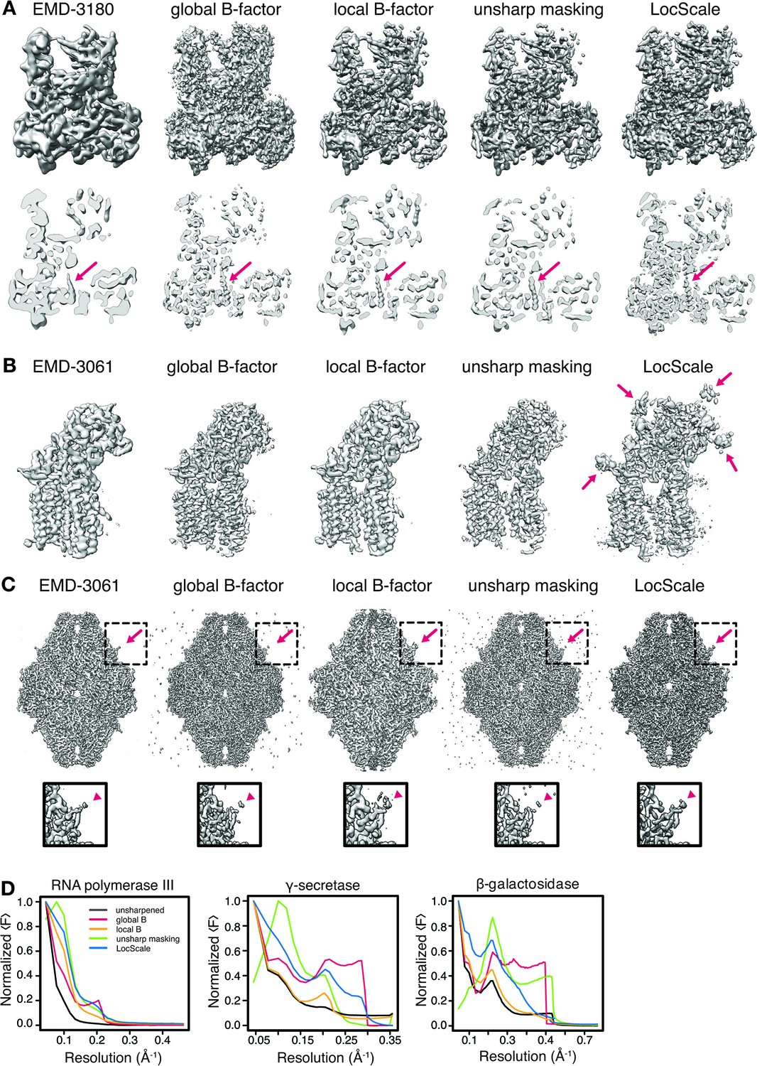
Comparison of global and local sharpening methods for Pol III, γ-secretase and β-galactosidase.
(A) Side view (top) and cross-section (bottom) of Pol III density maps obtained after sharpening with different sharpening methods as indicated. For comparison, detailed density features in the different maps are prominent for the central helix visible in the bottom part of the density map seen in the cross-section. In all cases (A–C) the left-most map represents the original 3D reconstruction before sharpening. Red arrows highlight density regions that are apparently different in the side view as an effect of the respective sharpening methods. (B) Comparison of sharpening methods applied to γ-secretase. (C) Comparison of sharpening methods applied to β-galactosidase. (D) Radial amplitude profiles for the maps shown in (A–C). The color coding in all cases follows that defined for Pol III (left).
Figure 3 with 3 supplements
Optimized cryo-EM map contrast by local model-based amplitude scaling (LocScale) and assessment of model bias.
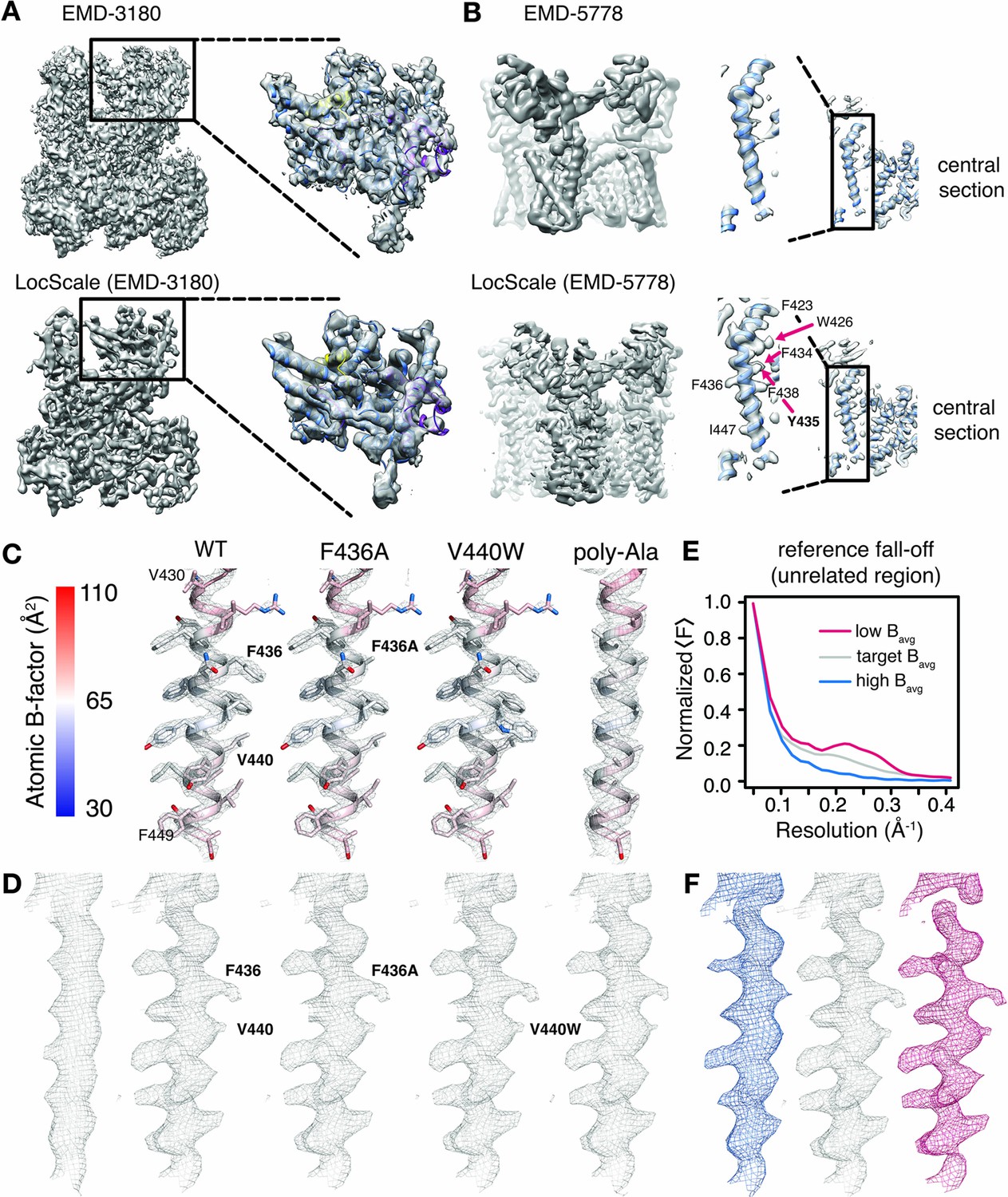
(A) and (B) Illustration of the LocScale sharpening for initially over-sharpened (A), RNA Pol III; EMD-3180) and under-sharpened maps (B,) TRPV1; EMD-5778). The maps after application of global (Guinier) sharpening (top) are shown in comparison with its LocScale equivalent (bottom). The LocScale map contains recognizable secondary structure. Zoomed-in inset: (A) The globally sharpened map shows undue noise amplification rather than true molecular features of the peripheral subunits as visualized in the LocScale map. Central section: (B) When global sharpening levels were underestimated, LocScale map reveals previously invisible features such as defined side chain densities (arrows). (C) Mesh representation of simulated reference densities for TRPV1 residues 430–449 for wild-type (WT), F436A, V440W and poly-alanine mutants superposed on the respective atomic model. Atoms are colored by atomic B-factor with B-factor scale as defined on the far left. (D) Mesh representation of density for residues 430–449 as deposited in EMD-5778 (far left) and LocScale maps obtained by sharpening using WT, F436A, V440W and poly-alanine mutants as a reference maps. The order follows that in (C). (E) Radial amplitude profile of a structurally unrelated region used as reference window for scaling with high (blue), target (grey) and low (red) average B-factors. The respective regions are shown in Figure 3—figure supplement 1. The denotation high and low refers to the average B-factor across the reference window compared with that estimated for the target window. (F) Densities for residues V420-F449 obtained after scaling using the reference falloffs in (E) with equivalent color-coding.
Figure 3—figure supplement 1
Assessment of coordinate and B-factor perturbation on LocScale densities and the relationship of atomic B-factors to local resolution.
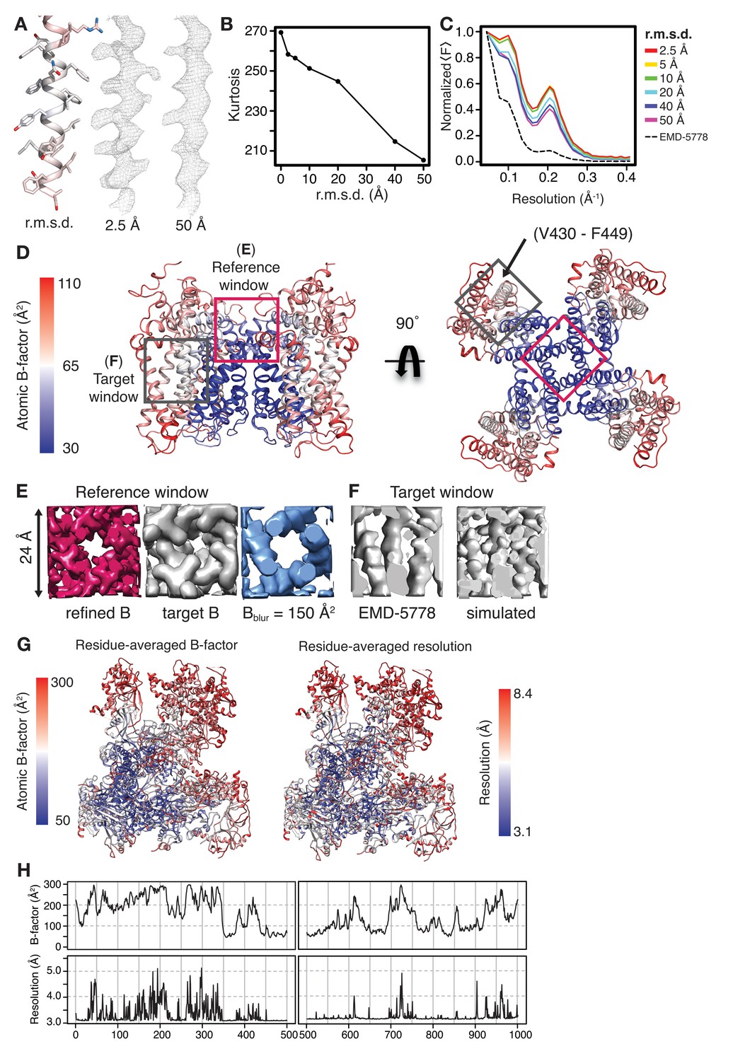
(A) Densities for TRPV1 residues V430-F449 (left, shown in cartoon/stick representation) obtained after perturbing initial coordinates of the reference model by 2.5 Å (middle) or 50 Å (right). Atoms in the unperturbed model (left) are colored according to B-factor as in (C). (B) Map kurtosis of LocScale maps as a function of coordinate perturbation (in Å r.m.s.d. from the initial coordinate model) used to compute the reference map for scaling. Kurtosis as a measure for sharpness of the map decreases with increasing model perturbation. (C) Radial amplitude profiles of the LocScale maps obtained after coordinate perturbation of the reference model. (D) Side (left) and top view (right) of the TRPV1 transmembrane region shown in cartoon representation. Regions used as reference (magenta) and target windows (grey) for scaling are highlighted by boxes. Atomic B-factors are mapped onto the cartoon model (scale bar shown on left). (E) Density for reference window shown in (D) simulated with the refined average B-factor from the atomic model contained in the reference window (left, magenta), simulated with the B-factor estimated for the target window from (D) (grey, middle) and simulated after blurring the refined B-factor by a 100 Å2 (blue, right). (F) Density for target window as in the unsharpened map (EMD-5778, left) and the corresponding density window simulated from the model in (D) (gray, right). (G) Comparison of residue-averaged B-factor (left) and local map resolution (right) mapped onto a cartoon representation of Pol III. The spatial distribution of atomic B-factors follows that of local resolution, with low B-factors (high resolution) in the core and high B-factors (low resolution) at the periphery. (H) Stacked diagrams of atomic B-factors (top) and local resolution (bottom) for two residue stretches of Pol III. Both quantities show correlating profiles of maxima and minima.
Figure 3—figure supplement 2
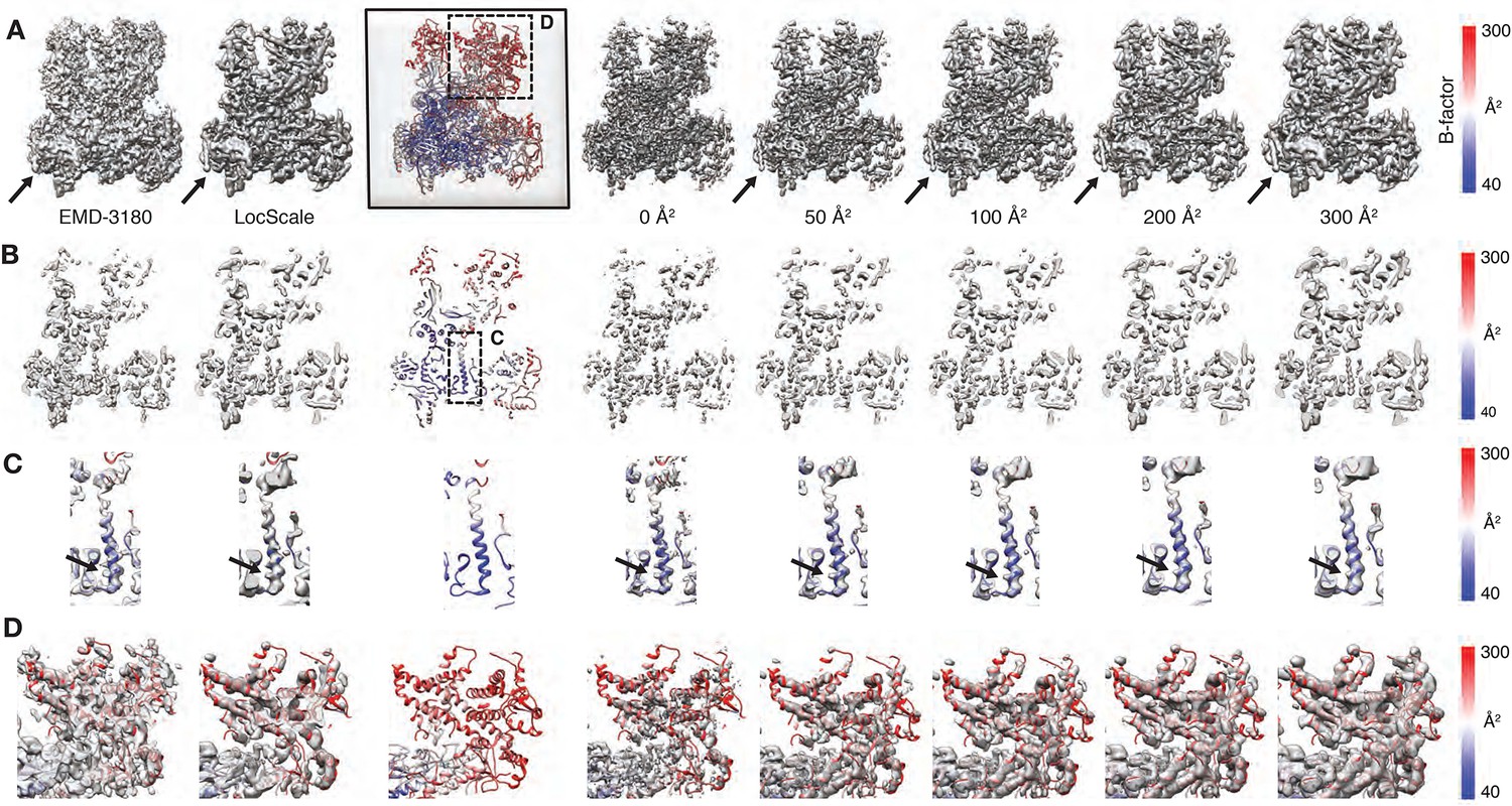
Effect of atomic B-factors on the LocScale procedure.
(A) Effect of atomic B-factors on the LocScale procedure. The atomic model (PDB ID 5fja) is shown in cartoon representation with residue-averaged B-factors as in defined by the scale bar (right). The deposited map (EMD-3180) and final LocScale map calculated using a reference map simulated from PDB ID 5fja are shown on the left. Right to the atomic model we show LocScale maps obtained with reference maps simulated from a coordinate model with uniform isotropic atomic B-factors of 0, 50, 100, 200 and 300 Å2, respectively. Each map element resolved at a particular resolution has a corresponding B-factor that best restores contrast in the respective LocScale map. (B) Central density slice for the presented densities in (A). (C) Close-up of a central helix with superimposed density. Note the progressive disappearance of side chain features in the LocScale maps (arrow) with atomic B-factors that are too high (≥200 Å2). (D) Close-up of a poorly resolved heterodimer region of Pol III as indicated in (A). When the average B-factor is too low (B = 0 Å2), peripheral helix map features become weak or fragmented. High B-factors (B = 300 Å2) lead to the appropriate low-pass filtered appearance of the same peripheral helix.
Figure 3—figure supplement 3
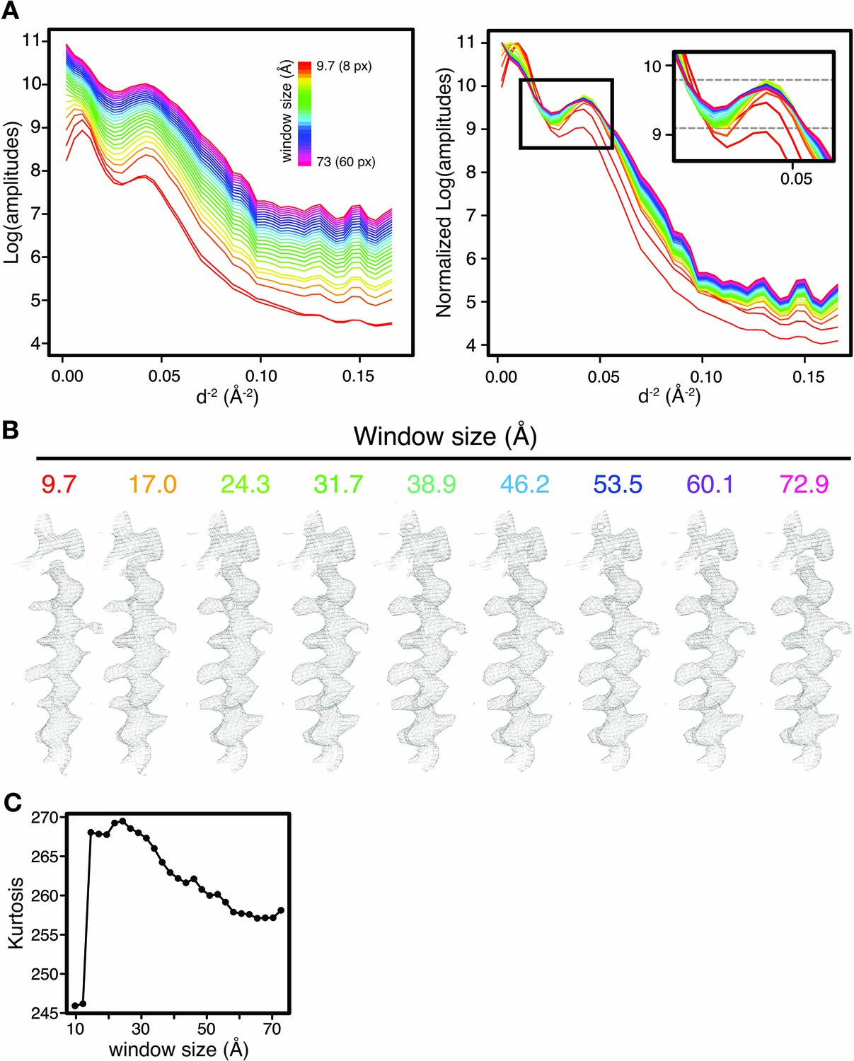
Effect of window size on local reference-based sharpening.
(A) Guinier plot of TRPV1 density (EMD-5778) obtained after LocScale sharpening with PDB 3j9j for window size ranging from 8 to 60 pixels (9.7–73 Å). (Left) Guinier profiles are colored in rainbow colours by window size as indicated. Note the increase in absolute scattering at zero spatial frequency with increasing window size. Also note the decreased amplitude at low resolution for small window sizes. (Right) Same profiles as shown left, scaled to the absolute frequency for the largest window, permitting comparison of Debye effect region at 7–4 Å (inset). The magnitude of the Debye effects first increases, then decreases with increasing window size. (B) LocScale densities for the V430-F449 transmembrane helix of TRPV1 shown for a selection of window sizes from (A). (C) Map kurtosis computed for the LocScale maps in (A). Kurtosis peaks for window sizes between 20–35 Å, corresponding to the range for which also Debye effects in (A) are found to be strongest.
Figure 4
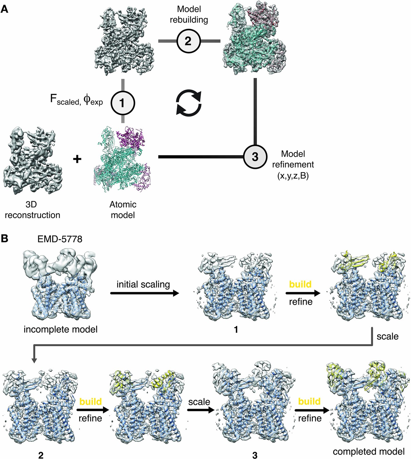
Cyclical workflow of iterative density sharpening using reference-based scaling and successive completion of atomic models.
(A) An atomic model is used as a reference to improve contrast in the original cryo-EM reconstruction employing local amplitude scaling (1). The resulting LocScale map contains improved contrast and thus facilitates further model building (2) and coordinate refinement (3). Scaling, building and refinement steps can be iterated to produce successively improved density maps and atomic models. (B) Workflow for extending atomic model beyond the reference structure using the LocScale procedure. (Top left) EM density for TRPV1 (EMD-5778) superposed onto an incomplete atomic model covering only the transmembrane region. In three successive cycles of LocScale sharpening and extension of the initial coordinate set by model building into new density with improved contrast, the atomic model can be completed to interpret the entire experimental density from EMD-5778. An effective window size of 25 Å was used for the LocScale iterations.
Figure 5 with 1 supplement
Application of the LocScale procedure to the 2.2 Å resolution cryo-EM structure of β-galactosidase and 3.4 Å structure of γ-secretase.
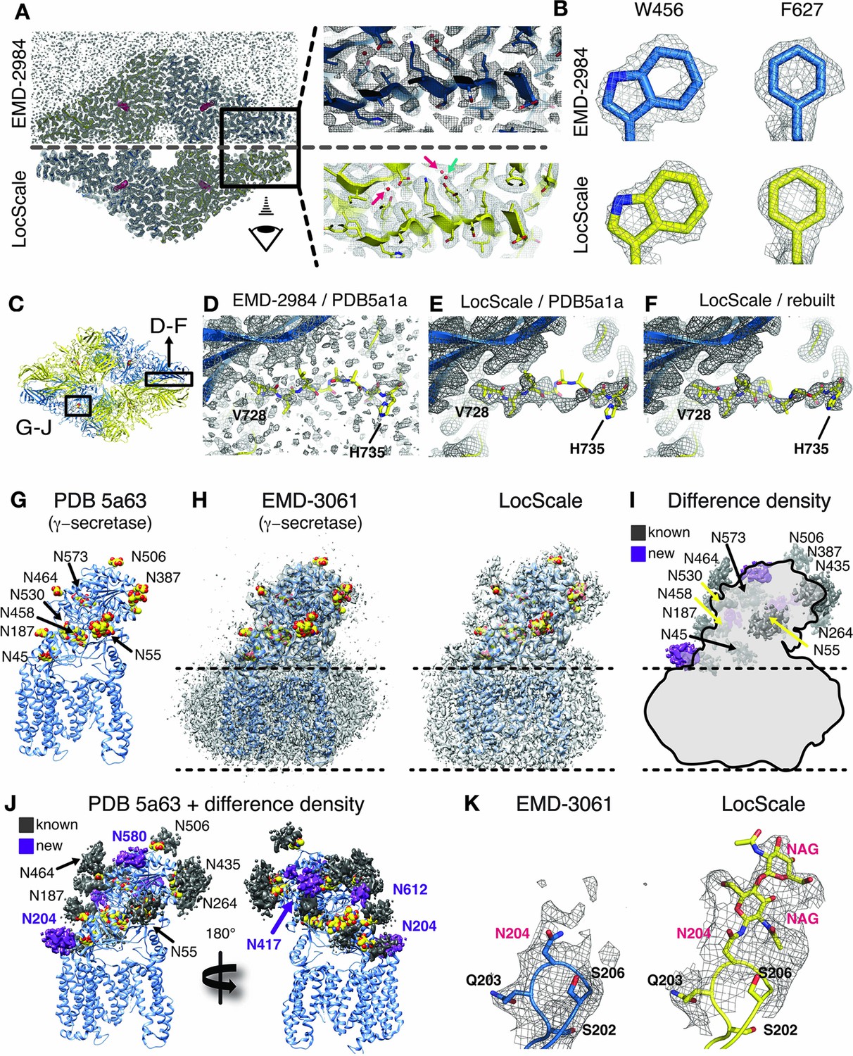
(A) Overall comparison of uniformly sharpened (EMD-2984) (top) and LocScale map (bottom) for the β-galactosidase structure. EMD-2984 displays visible noise at the periphery of the molecule and its surrounding solvent, whereas the LocScale map contains reduced noise levels in corresponding regions. Zoomed-in regions in the protein core showing modeled water molecules for which density is retained in the LocScale map (arrows). (B) High-resolution details such as doughnut-shaped densities for aromatic side chains W456 and F627 in the EMD-2984 map (top) are consistently retained in the LocScale map (bottom). Maps are shown at equivalent isosurface levels displayed at a 1.6 Å carve radius. (C) Cartoon representation of the β-galactosidase tetramer (PDB ID 5a1a) colored by symmetry-related subunits (yellow and blue). (D–F) Density around the peripheral loop region comprising residues V728– H735 (see (C) for overall location) fragmented in the deposited map, hampering unambiguous tracing of the backbone conformation. Deposited conformation in PDB ID 5a1a superimposed on the EMD-2984 map (D) and LocScale map (E). Note reduced noise levels and continuous density providing an unambiguous backbone trace in the LocScale map. The LocScale density is not compatible with the modelled conformation of PDB ID 5a1a, but supports an alternative conformation of V728–H735 shown superimposed on the LocScale map (F). (G) Atomic model of γ-secretase (PDB ID 5a63) in cartoon representation. Modeled glycan residues in nicastrin are shown as spheres and N-linked glycosylation sites are indicated. (H) Comparison of EMD-3061 (left) and LocScale (right) maps contoured at 3σ with ribbon model as in (G). (I) Difference density of (H left and right) superposed on light gray silhouette representation of EMD-3061. Regions with difference density beyond 4σ located at known glycosylation sites are colored in dark gray and newly identified glycosylation sites are shown in purple. (J) Difference density from (I) mapped onto the atomic model of γ-secretase. Purple difference density locates to putative additional glycosylation sites. (K) Density around N204 of nicastrin for EMD-3061 (left) and LocScale map (right) reveals additional density for two N-acetylglucsoamine (NAG) residues in the LocScale map.
Figure 5—figure supplement 1
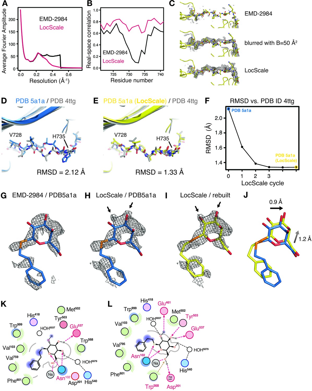
Comparison of β-galactosidase radial amplitude profiles and iterative refinement of coordinates from the V728–H735 loop region.
(A) Radial amplitude spectrum of LocScale β-galactosidase map. In comparison with the deposited map obtained by uniform B-factor sharpening, the LocScale procedure results in a smooth falloff to high-resolution amplitudes. (B) Residue-based real-space correlation improves in the V728–H735 loop region for the conformation built using the LocScale map. (C) Comparison of density for the V728–H735 region in EMD-2984 (top), EMD-2984 after blurring with a B-factor of 50 Å2 and the LocScale map for EMD-2984 (bottom). Maps are contoured at 3σ and displayed with a carve radius of 2.0 Å. (D) Comparison of the V728–H735 stretch of PDB ID 5a1a (blue) with the 1.6 Å crystal structure of E.coli β-galactosidase PDB ID 4ttg (silver). The RMSD states the root mean square deviation between PDB IDs 5a1a and 4ttg computed across all atoms in the sequence V728–H735. (E) Same view as (C) comparing the model after rebuilding and iterative refinement using the LocScale procedure (yellow). (F) Plot of the model differences in RMSD (Å) illustrated in (C) and (D) as a function of alternating LocScale and refinement cycle. (G–J) Density for the PETG ligand bound in the active site as observed in EMD-2984 (G) and LocScale map (H) superposed on the PETG conformation from PDB ID 5fja shown in stick representation. Enhanced density features of the hydroxyl substituents in the hexapyranosyl ring become visible in the LocScale map (arrows) and require re-arrangement of the ligand orientation in the active site (I and J). (K and L) FLEV ligand environment computed from PDB ID (5fja) and the model after refinement against the LocScale map. Re-orientation of the ligand based on the LocScale map increases hydrogen-bond interactions in the active site. Note also the significantly decreased substitution contour (gray line) for the LocScale conformation, indicating tighter apposition in the active site.
Figure 6 with 2 supplements
Effect of local sharpening on RNA density in the ribosome EF-Tu complex.
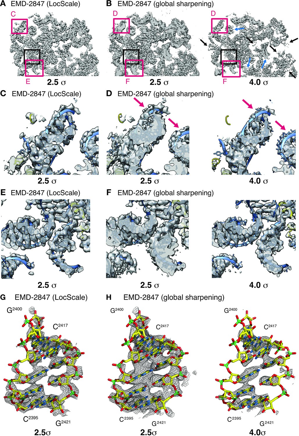
(A) Cross-section through cryo-EM density of the E.coli ribosome EF-Tu complex (EMD-2847) after local sharpening with LocScale contoured at 2.5 σ. Red frames correspond to density enlarged in panels C and E whereas black frame corresponds to density in G. All parts of the LocScale map are interpretable at a single density threshold level. (B) Cross-section as in (A) after sharpening with a global B-factor contoured at 2.5 σ (left) and 4.0 σ (right). Not all parts of the maps are equally interpretable at 2.5 σ. Strong density sections reveal increased detail at higher threshold levels (blue arrows). In turn, weaker parts of the map are no longer visible at these threshold levels (black arrows). (C) Close-up of LocScale density displaying a peripheral ribosomal RNA fragment as indicated in (A). RNA density including nucleotide bases and the phosphate backbone is visible (blue ribbon) and base stacking is partially recognizable along the RNA strand. In addition, protein density (yellow ribbon) is visible when contoured at 2.5 σ. (D) Same area as in (C), here displayed for the globally sharpened map contoured at 2.5 σ (left) and 4.0 σ (right). Visualization at increased density threshold is required to reveal additional detail on nucleotide base stacking, at the expense of density for phosphate backbone (arrows) and adjacent protein components. (E) Close-up of LocScale density displaying a well-resolved ribosomal RNA fragment as indicated in (A). Nucleotide base stacking is recognizable in all displayed RNA duplexes. (F) Same area as in (E) displayed for the globally sharpened map contoured at 2.5 σ (left) and 4.0 σ (right). (G) LocScale density: detailed view on a ribosomal RNA fragment (shown in stick representation; N (blue) O (red), C (yellow), P (green)) for EMD-2847. The density is contoured at 2.5 σ. (H) Globally sharpened density: same RNA fragment as in (G) for EMD-2847 contoured at 2.5 σ (left) and 4.0 σ. Simultaneously resolving nucleotide base stacking and phosphate backbone at a single threshold level is not possible. A carve radius of 2.5 Å was used for density representations in G and H.
Figure 6—figure supplement 1
Effect of local sharpening on threshold level and map interpretability of maps with resolution variation illustrated for RNA Pol III.
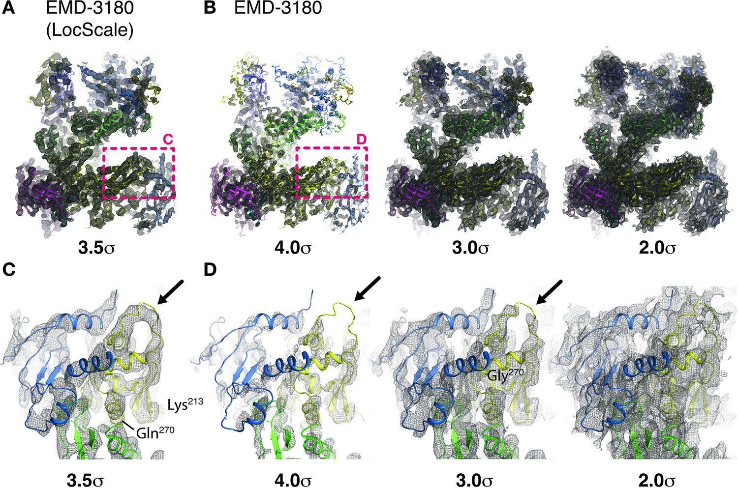
(A) Locally sharpened (LocScale) map of RNA Pol III (EMD-3180) contoured at 3.5 σ. All parts of this maps are visible and interpretable at a single threshold. (B) Globally sharpened map of RNA Pol III (EMD-3180) contoured at 4.0 σ (left), 3.0 σ (middle) and 2.0 σ (right). Multiple different threshold levels are required to visualize and interpret central and peripheral parts of the map. (C) Selected LocScale density fragment (indicated in (A)) of the RNA Pol III map contoured 3.5 σ and superposed onto the atomic model (PDB ID 5fja). Note the continuous density for the loop region indicated by the arrow. The LocScale map suggests that the conformation of this loop region in the deposited model does not match the density optimally. RPC1 (green), RPC2 (yellow), RPC5 (purple) are shown in cartoon representation. (D) Same density fragment as in (C, indicated in (B)) now shown for the globally sharpened RNA Pol III map (EMD-3180) contoured at 4.0 σ (left), 3.0 σ (middle) and 2.0 σ (right). The weak density of full loop region (arrows) is only visible at low threshold, where other parts of stronger density now start to cover up the loop density, reducing clarity and hampering confident modeling of the displayed region.
Figure 6—figure supplement 2
Effect of local sharpening on peripheral density in the 20 s proteasome.
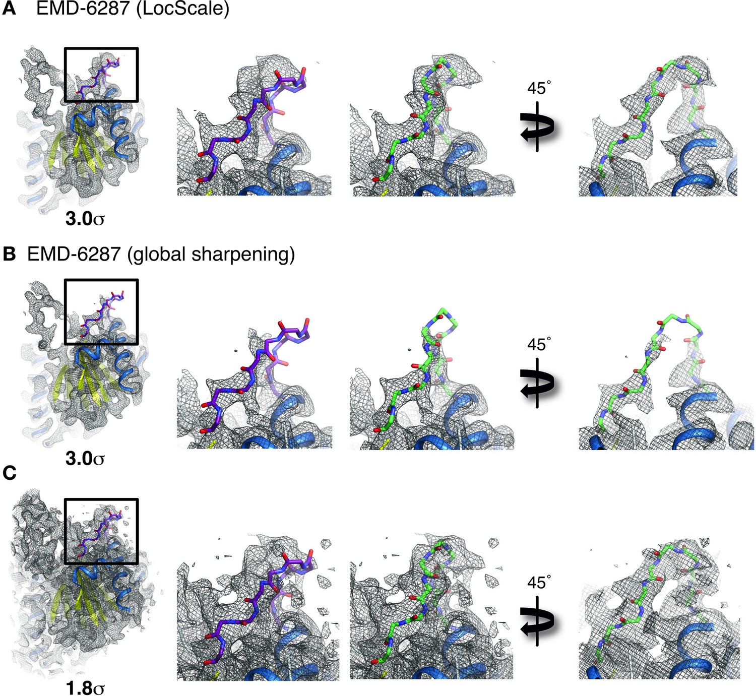
(A) Cartoon representation of 20 s proteasome monomer (left; PDB ID 1y7t) superposed onto LocScale density for EMD-6287. A poorly resolved peripheral loop region is shown in stick representation. A close-up of the peripheral loop region reveals that the LocScale density is incompatible with the loop conformation of the crystal structure of PDB ID 1y7t (purple, middle left). Refinement against the LocScale map yields a different conformation that is in better agreement with the EM density (green, middle right). Density is contoured at 3.0 σ. (B) Cartoon representation of 20 s proteasome monomer (left; PDB ID 1y7t) superposed onto globally sharpened density for EMD-6287. As expected for a map with modest local resolution variation, nearly all of the density is similarly well visualized as in the LocScale map. No density is visible for the peripheral loop region at the 3.0 σ contour, allowing no distinction between the different conformations from (A). (C) Lowering the density threshold to 1.8 σ reveals additional density for the peripheral loop compatible with the conformation obtained from refinement against the LocScale map (green). At this density threshold level detail for other parts of the map becomes obscured.
Figure 7 with 2 supplements
Details of LocScale maps for TRPV1 and RNA Pol III.
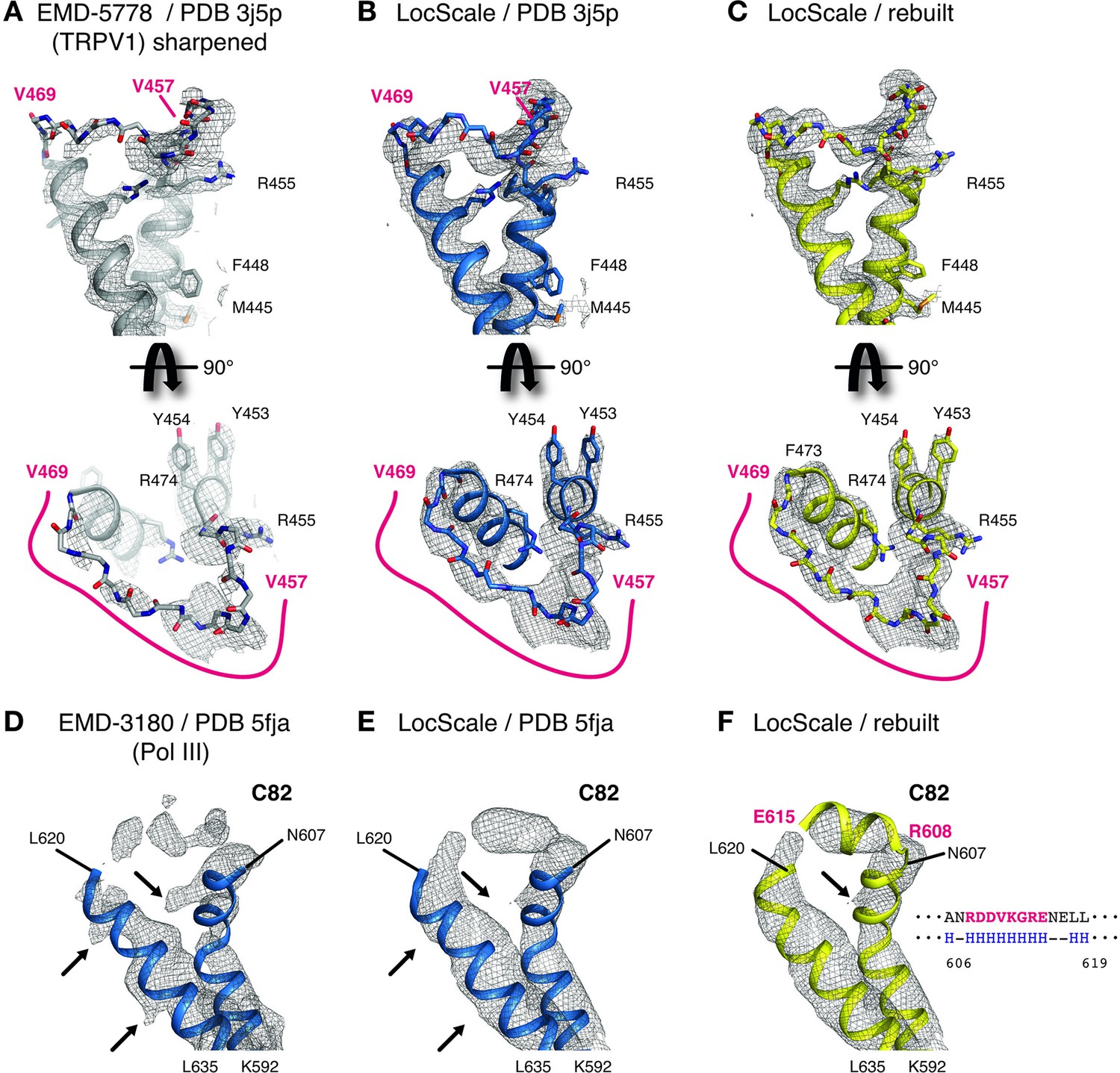
(A) Close-up density for TRPV1 channel (EMD-5778) superposed on the deposited coordinate model (PDB ID 3j5p). The map was additionally sharpened with a B-factor of −100 Å2 to make densities for aromatic and other large side chains more clearly visible. Transmembrane views (top) and the corresponding perpendicular view (bottom) of the V457–V469 loop region are displayed, showing poorly resolved density for V457–V469 residues (main chain shown in stick representation). Selected residues with large side chains are also shown in stick representation. (B) Same view as (A) with PDB ID 3j5p superposed onto the LocScale density. Density is shown at a threshold level matching visible side-chain densities in (A). Continuous density is observed for residues V457–V469, allowing less ambiguous building of the main chain trace. (C) LocScale density for the same regions shown in (A) and (B) superposed on the atomic model obtained after adjustment and refinement against the LocScale map. (D) Close-up density for Pol III subunit C82 (EMD-3180) superposed onto the deposited atomic model (PDB 5fja) shown in cartoon representation. Density for residues R608–L619 is fragmented and precludes model building. Note the pronounced density artifacts (arrows) incompatible with side chain densities. (E) Same view as (D) with PDB 5fja superposed onto the LocScale density. The density is suggestive of a helical conformation for residues R608-E615, confirming secondary structure predictions (right). Density artifacts from (D) are reduced in the LocScale map. (F) C82 model rebuilt and refined using the LocScale map. The predicted helix formed by residues R608-E615 fits the helical density as suggested by the LocScale map.
Figure 7—figure supplement 1
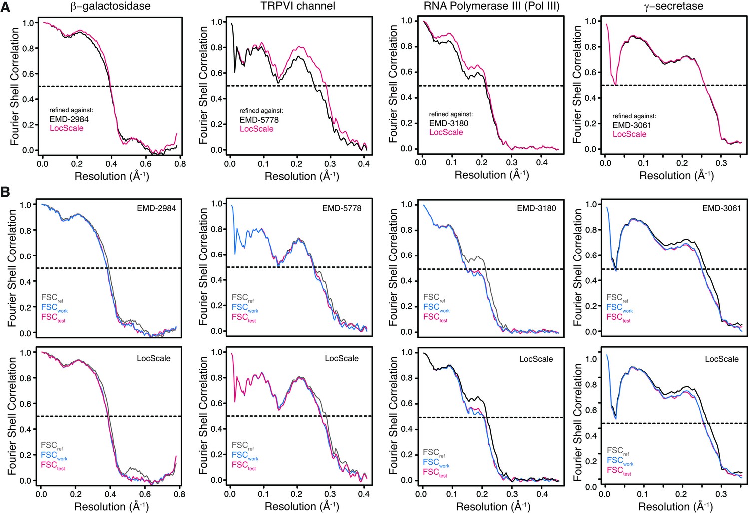
Model validation.
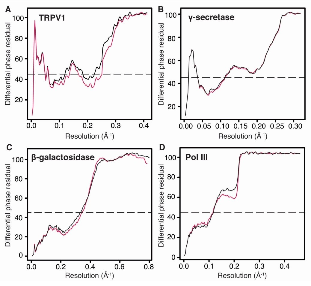
(A) FSCref curves for β-galactosidase, TRPV1, Pol III and γ-secretase models refined against the original EMDB entry (black) or the respective LocScale map (red). All FSCref curves were computed using the original density map. (B) FSC curves for work (FSCwork, blue) and cross-validated test maps (FSCtest, red) from model refinement and validation using independent half maps shown for both refinement against the original PDB entry (top) and the respective LocScale maps (bottom). The closely matching profiles of FSCwork and FSCtest indicates that no significant overfitting took place. The corresponding FSCref (gray) are shown for comparison.
Figure 7—figure supplement 2
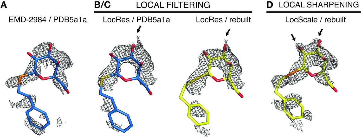
LocScale maps recover contrast better when compared with local resolution-filtered (LocRes) maps.
(A) Density for the PETG ligand bound in EMD-2984 superposed on the PETG conformation from PDB ID 5fja shown in stick representation (replicate from Figure 4G). All densities are carved around the PETG ligand with a 1.6 Å carve radius. (B–C) PETG from PDB ID 5fja (B) or the model obtained after refinement against the LocScale map (C) superposed on the density of EMD-2984 filtered according to local resolution (LocRes). (D) LocScale density with PETG ligand as in Figure 4J. The LocScale map recovers density contrast to reveal the hydroxyl substituents of the hexa-pyranosyl ring.
Author response image 1
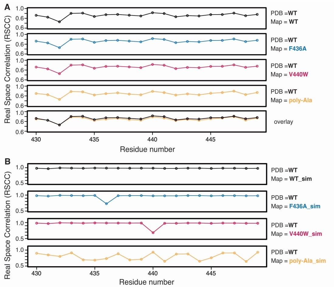
Quantification of reference model perturbation on LocScale maps.
(A) Residue-averaged real space correlation (RSCC) for TRPV1 residues 430-449 computed between the original PDB (WT) and LocScale maps obtained with scaling using a WT, F436A, V440W or poly-Ala reference map. (B) Residue-averaged real space correlation (RSCC) for TRPV1 residues 430-449 computed between the original PDB (WT) and the simulated reference maps obtained from WT, F436A, V440W or poly-Ala coordinate models.
Author response image 2
Tables
Table 1
Model refinement statistics
https://doi.org/10.7554/eLife.27131.020| β-galactosidase (Bartesaghi et al., 2015) | TRPV1 Channel (Liao et al., 2013) | RNA polymerase III (Hoffmann et al., 2015) | γ-secretase (Bai et al., 2015) | |||||
|---|---|---|---|---|---|---|---|---|
| EMD-2984 | LocScale | EMD-5778 | LocScale | EMD-3180 | LocScale | EMD-3061 | LocScale | |
| Starting model PDB ID | 5a1a | 3j5p | 5fja | 5a63 | ||||
| Resolution (Å) LocRes range (Å) | 2.2 (1.9–3.6) | 3.4 (2.5–4.8) | 4.7 (3.4–8.1) | 3.4 (3.0–6.8) | ||||
| Refinement (Å) | 186.0–1.9 | 311.3–2.5 | 320.9–3.4 | 252.0–3.0 | ||||
| Overall RSCC* | 0.70 | 0.75 | 0.62 (0.75)§ | 0.67 (0.81)§ | 0.70 | 0.76 | 0.71 | 0.77 |
| EMRinger score† | 4.03 | 4.90 | 0.24 | 0.77 | 2.60 | 2.87 | ||
| MOLPROBITY score | 2.04 | 1.86 | 2.69 (1.44)§ | 1.98 (1.35) | 2.68 | 2.24 | 2.01 | 1.81 |
| Clash score‡ (all atoms) | 6.63 | 3.14 | 6.88 (2.42)§ | 5.29 (2.09)§ | 16.44 | 11.04 | 6.44 | 5.89 |
| Rotamer outliers (%) | 3.32 | 4.92 | 16.38 (0.00)§ | 2.23 (0.00)§ | 2.53 | 1.48 | 1.53 | 0.86 |
| Ramachandran statistics Favored (%) Disallowed (%) | 95.98 0.00 | 96.57 0.00 | 94.3 (93.6)§ 0.35 (0.64)§ | 93.4 (94.6)§ 0.17 (0.64)§ | 83.2 1.09 | 85.4 0.99 | 92.86 0.33 | 91.74 0.33 |
| RMS bonds (Å) | 0.008 | 0.01 | 0.008 | 0.006 | 0.008 | 0.01 | 0.011 | 0.012 |
| RMS angles (°) | 1.41 | 1.50 | 1.71 | 1.44 | 1.67 | 1.32 | 1.41 | 1.53 |
-
*Overall real-space correlation computed at the average map resolution using a soft mask around atoms. The EMDB deposition was used as the reference map in all cases.
†EMRinger score calculated only for parts of structure with local resolution estimate better than 4.5 Å.
-
‡Clash score denotes number of van der Waals overlap per 100 atoms.
§EMRinger scores in brackets are reported for the transmembrane region.
Table 2
Model refinement statistics for local resolution-filtered maps.
https://doi.org/10.7554/eLife.27131.021| β-galactosidase | TRPV1 channel | RNA polymerase III | γ-secretase | |
|---|---|---|---|---|
| LocRes | LocRes | LocRes | LocRes | |
| Starting model PDB ID | 5a1a | 3j5p | 5fja | 5a63 |
| Resolution (Å) LocRes range (Å) | 2.2 (1.9–3.6) | 3.4 (2.5–4.8) | 4.7 (3.4–8.1) | 3.4 (3.0–6.8) |
| Refinement (Å) | 186.0–1.9 | 311.3–2.5 | 320.9–3.4 | 252.0–3.0 |
| Overall RSCC* | 0.72 | 0.64 (0.78)§ | 0.72 | 0.73 |
| EMRinger score† | 4.15 | 0.46 | 0.89† | 2.69 |
| MOLPROBITY score | 2.00 | 2.43 (1.40)§ | 2.62 | 1.95 |
| Clash score‡ (all atoms) | 4.45 | 6.45 (2.34)§ | 13.31 | 6.18 |
| Rotamer outliers (%) | 3.83 | 4.63 (0.00)§ | 1.95 | 1.00 |
| Ramachandran statistics Favored (%) Disallowed (%) | 96.24 0.00 | 95.1 (94.9) 0.31 (0.64)§ | 86.4 1.00 | 93.01 0.48 |
| RMS bonds (Å) | 0.008 | 0.008 | 0.01 | 0.01 |
| RMS angles (°) | 1.48 | 1.43 | 1.42 | 1.50 |
-
*Overall real-space correlation computed at the average map resolution using a soft mask around atoms. The EMDB deposition was used as the reference map in all cases.
†EMRinger score calculated only for parts of structure with local resolution estimate better than 4.5 Å.
-
‡Clash score denotes number of van der Waals overlaps per 100 atoms.
§Scores in brackets are reported for the transmembrane region.
Additional files
-
Transparent reporting form
- https://doi.org/10.7554/eLife.27131.022
Download links
A two-part list of links to download the article, or parts of the article, in various formats.
Downloads (link to download the article as PDF)
Open citations (links to open the citations from this article in various online reference manager services)
Cite this article (links to download the citations from this article in formats compatible with various reference manager tools)
Model-based local density sharpening of cryo-EM maps
eLife 6:e27131.
https://doi.org/10.7554/eLife.27131


