A predictive model of asymmetric morphogenesis from 3D reconstructions of mouse heart looping dynamics
- Laboratory of Heart Morphogenesis, France
- Université Paris Descartes, France
- University of Jaén, CU Las Lagunillas, Spain
- Centro Nacional de Investigaciones Cardiovasculares, CNIC, Spain
- University of East Anglia, United Kingdom
- Norwich Research Park, United Kingdom
- The Francis Crick Institute, United Kingdom
Figures
Figure 1
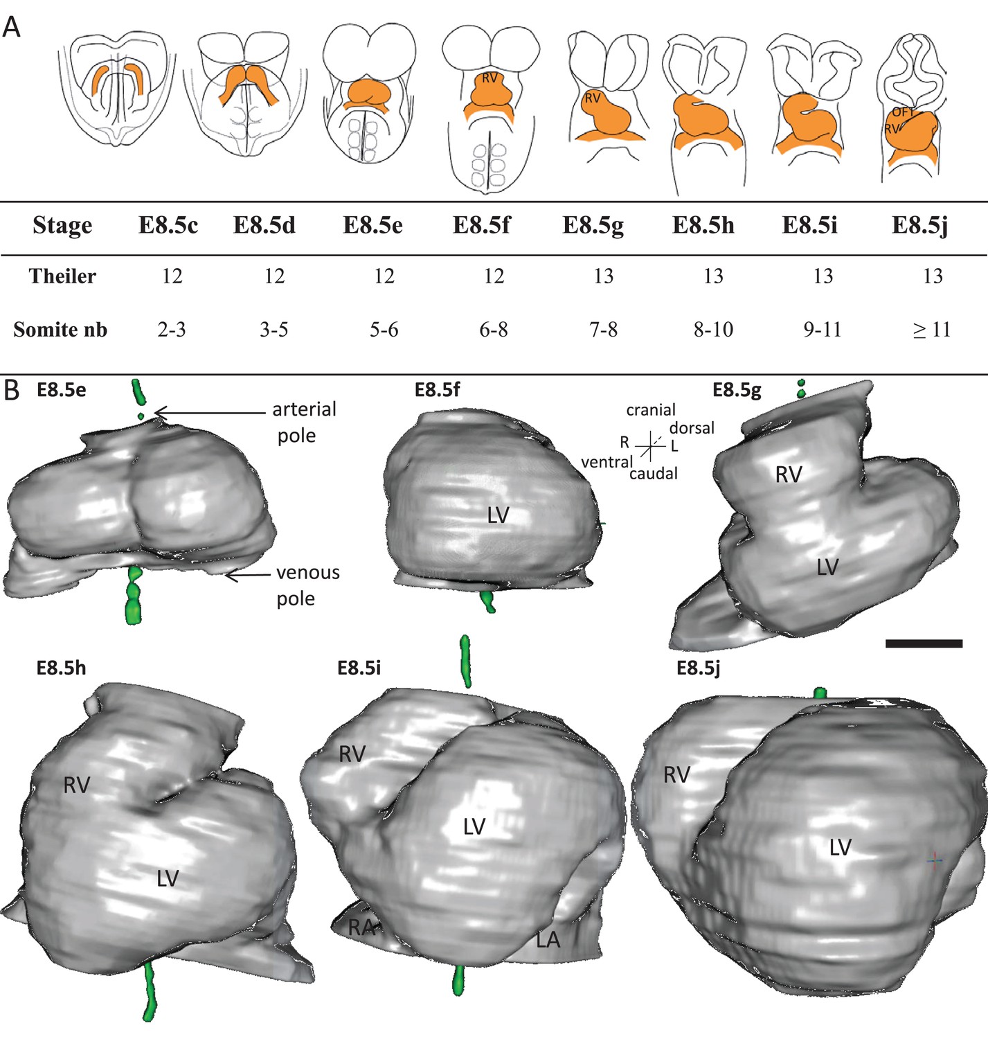
Stages depicting the progression of heart looping in the mouse.
(A) Schematic representation of shape changes during the formation and looping of the heart tube (orange) in the E8.5 mouse embryo. Until E8.5f, the mouse embryo appears bilaterally symmetrical, and the heart tube is straight. The staging scale goes from E8.5c to E8.5j (previous E8.5a-b stages are not shown). This scale, focused on the heart, is finer than Theiler stages, and not fully synchronous with the addition of somites. Somite numbers (nb) were counted in a collection of 40 embryos imaged by HREM between E8.5e and E8.5j and of 48 embryos between E8.5c and E8.5d observed under the microscope. (B). 3D reconstructions of heart shapes from HREM images at each stage of heart looping. All the reconstructions are aligned with the notochord vertical (green), the arterial and venous poles up and down, respectively. L, left; LA, left atrium; LV, left ventricle; OFT, outflow tract; R, right; RA, right atrium; RV, right ventricle. Scale bar: 100 μm.
-
Figure 1—source data 1
3D reconstructions of heart stages during the looping process, in a 3D pdf format.
3D visualisation of the heart, as reconstructed from HREM images, at the six stages shown in Figure 1. This file should be opened with Adobe Acrobat Reader. Click on the image to activate the manual rotation of the reconstruction. Each image may be rotated at will with the mouse (hold left click). Zoom in and out with the mouse wheel. Shortcuts at the top align all images in a ventral or dorsal view, with the notochord vertical.
- https://doi.org/10.7554/eLife.28951.004
Figure 2
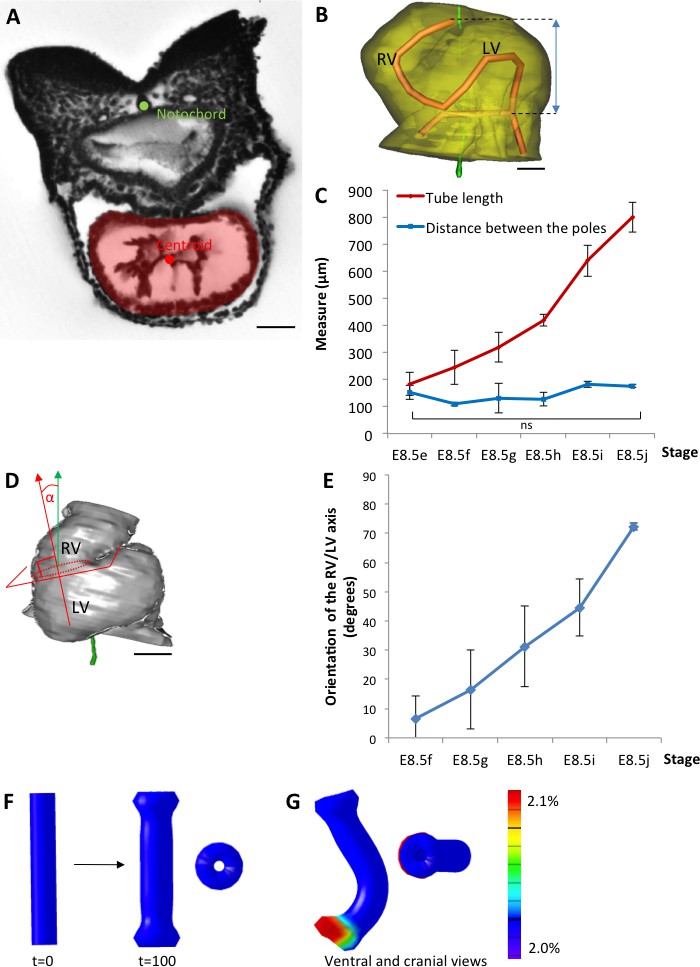
The heart tube elongates and loops between fixed poles.
(A) HREM image of an embryo section at E8.5f, with the notochord (green dot) and the centroid (red dot) of the myocardial tube (pale red) outlined. (B) Ventral view of a 3D reconstruction of the heart tube at E8.5i, aligned with the notochord vertical (green), showing the axis of the myocardial tube (red) used for the measurement of its length, and the distance between its poles (blue double-arrow). The measures were taken between the top of the arterial pole and the bifurcation between the two atrial regions at the venous pole. The distance between the poles was measured after projection onto the notochord. (C) Comparison between the tube length (red) and the distance between the poles (blue) during heart development. (D) Ventral view of a 3D reconstruction of the heart tube at E8.5h, aligned with the notochord vertical (green), showing the measurement of the orientation of the right ventricle (RV)-left ventricle (LV) axis. The perpendicular (red arrow) to the section of the interventricular sulcus (dotted circle) was drawn and its angle with the notochord (green arrow) was calculated. The measure was taken after projection onto the frontal plane. (E) Inclination of the right ventricle (RV)-left ventricle (LV) axis when looping progresses from a cranio-caudal (0°) towards a left-right orientation (90°). (F) Computer simulation of shape changes, in 3D, with a Finite Element model, seen from ventral (left) and cranial (right) views at step 100. Starting from a straight tube (t = 0), the simulation was run under the hypothesis of a tube growing homogenously between fixed poles, in the absence of any asymmetry. (G) Similar computer simulation, but with a small (5%) left-right asymmetry at one pole, mimicking stochastic, naturally occurring, left-right variations. The coloured scale of longitudinal growth used in the simulations is indicated on the right. Means and standard deviations are shown, with n = 3 for each point. Scale bar: 50 μm (A,B), 100 µm (D).
Figure 3
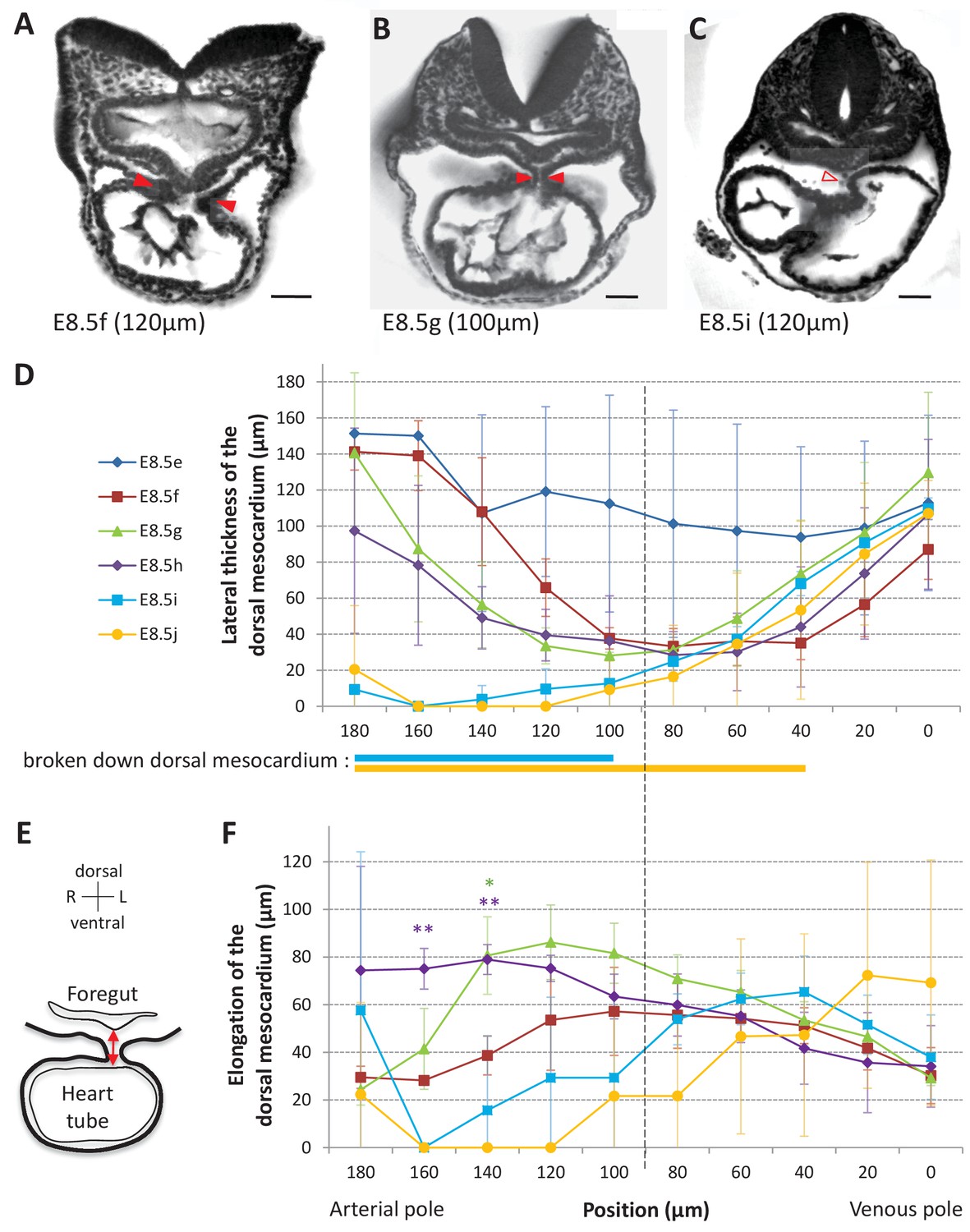
Progression of dorsal mesocardium breakdown during heart looping.
(A) Transverse section from an HREM image of an embryo at E8.5f showing the attachment of the heart tube to the body via the dorsal mesocardium (lateral thickness between red arrowheads). The position, along the notochord, of the section is indicated in brackets, as the distance to the bifurcation between the two atrial regions. (B) At equidistance between the poles at E8.5g, the dorsal mesocardium is thinner (red arrowheads). (C) In the arterial half of the tube at E8.5i, the dorsal mesocardium is broken down (open arrowhead). (D) Measure of the lateral thickness of the dorsal mesocardium, in serial positions along the notochord, from the arterial pole (left) to the venous pole (right), at successive developmental stages (colour coded). Thick lines below indicate positions where at least one sample had dorsal mesocardium breakdown. The boundary between the arterial and venous halves of the tube is shown by a vertical dashed line. (E) Schematic representation of a transverse section, showing the dorso-ventral elongation of the dorsal mesocardium (red double arrow), measured as the distance to the ventral fold of the foregut. (F) Measure of the elongation of the dorsal mesocardium, in serial positions along the notochord at successive developmental stages (colour coded). A significant elongation of the dorsal mesocardium, compared to the initial heart tube at E8.5f, is indicated by asterisks (*p-value<0.05 and **p-value<0.01, two-tailed Student test). When the dorsal mesocardium has broken down, the elongation value is set to 0. Means and standard deviations are shown (n = 3 for each stage). Scale bars: 50 μm.
Figure 4 with 1 supplement
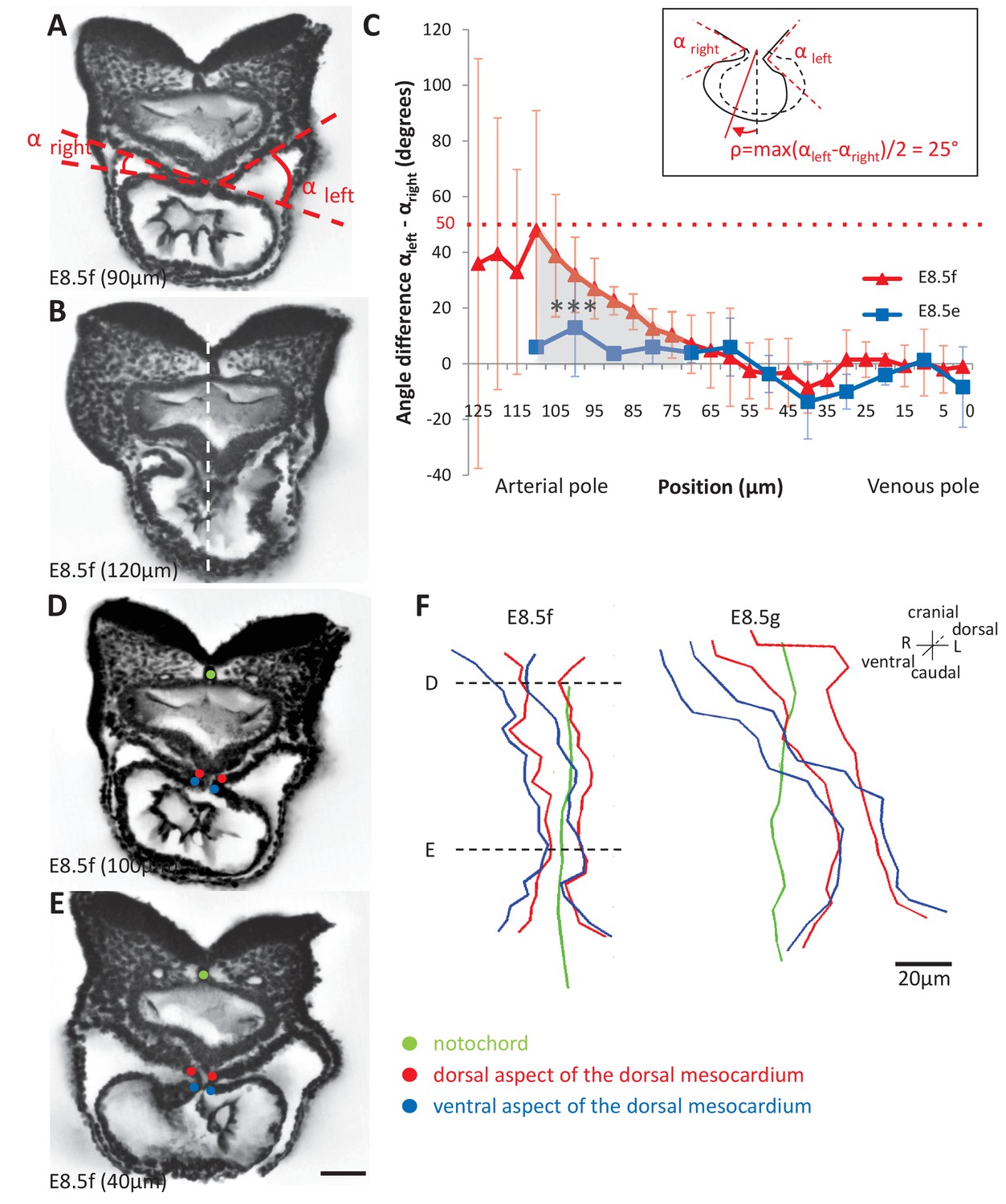
Rotation of the arterial pole at E8.5f.
(A) Transverse section from an HREM image of an embryo at E8.5f, in which the angles (right and left) between the heart tube and the dorsal pericardial wall, at the dorsal mesocardium, are shown. The position of the section is indicated in brackets, as a distance to the bifurcation between the two atrial regions. (B) Section of the same heart at the arterial pole, showing the asymmetry of the tube relative to the dorsal-ventral axis of the embryo (white dashed line). (C) Quantification of the left-right difference between the angles at the dorsal mesocardium, taken at successive positions along the axis of the notochord. A significant difference (***p-value<0.001, paired Student test) at the arterial pole at E8.5f is indicated in grey. From the maximum value of the angular difference, we can estimate the angle of rotation (ρ) of the tube relative to the dorsal-ventral axis (see inset). Means and standard deviations are shown (n = 3 for each stage). (D–E) Transverse embryo sections at E8.5f, at the arterial pole (D) and venous pole (E), with the notochord (green) and the dorsal (red) and ventral (blue) aspects of the dorsal mesocardium outlined. (F) In representative embryos, ventral views, aligned with the notochord, of the position of the dorsal mesocardium along the arterial (top) - venous (down) axis of the tube. The position of the sections in (D) and (E) is indicated. Scale bars: 50 µm (A, B, D, E), 20 µm (F).
Figure 4—figure supplement 1
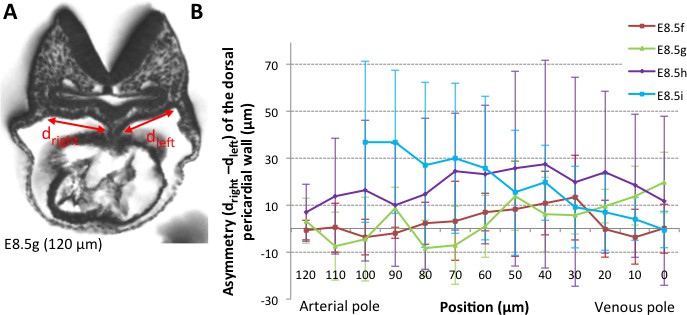
Asymmetry of the dorsal pericardial wall.
(A) Transverse embryo section at E8.5g, in which the width of the dorsal pericardial wall on either sides of the dorsal mesocardium is shown. The position of the section is indicated in brackets, as the distance to the bifurcation between the two atrial regions. (B) Quantification of the left-right difference between the widths, in serial positions along the notochord and at successive developmental stages (colour coded). No significant difference between the left and right is detected (Student paired test, p>0.27 at E8.5f, >0.12 at E8.5g, >0.23 at E8.5h and p>0.09 at E8.5i). Means and standard deviations are shown, with n = 3 at E8.5f-h, 4 at E8.5i.
Figure 5
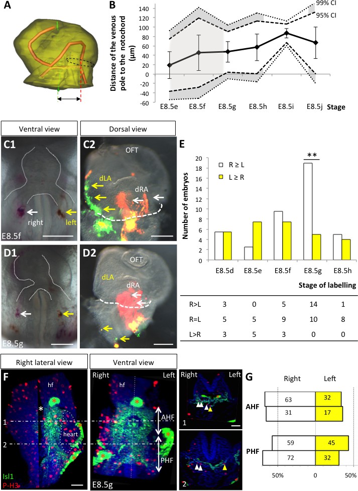
Asymmetric cell ingression at the venous pole at E8.5g.
(A) 3D reconstruction of the heart tube at E8.5i, aligned with the notochord vertical (green), showing the axis of the myocardial tube (red) and the last tube section before the bifurcation (dotted black line) used for the measurement of the position of the venous pole. The distance to the notochord (double black arrow) was measured after projection onto the frontal plane. (B) Displacement of the venous pole during the looping process. Positive values indicate a leftward deviation, which we take as significant when the null value (0) lies outside the 95% confidence interval (CI) at E8.5g-h and E8.5i, and outside the 99% confidence interval at E8.5i. Means and standard deviations are shown, with n = 3 at E8.5e-h and 4 at E8.5i-j. (C1–D1) Brightfield images (ventral view) of embryos at the indicated stage, showing the symmetrical DiI and DiO labelling in the right (white arrow) and left (yellow arrow) posterior heart field, respectively. The contour of the heart tube is outlined (dotted white line). (C2–D2) Fluorescent signal on brightfield images (dorsal view) of the isolated heart after 24 hr of embryo culture, in which the labelled regions deriving from the right (white arrows) and left (yellow arrows) injections are visible. The boundary of the heart tube is indicated (dashed white line), showing that both labelled regions are within the heart tube in C2, whereas this is the case only for the right label in D2. (E) Quantification of left-right differences in the ingression of cells from the posterior heart field. At each stage of labelling, the number of embryos, in which the right (white) or left (yellow) label had progressed further into the heart tube after 24 hr of culture, is indicated. Embryos in which no obvious asymmetry between the right and left was observed were equally distributed in the two other categories. A significant difference is observed at E8.5g only (chi-square test with Yates’ correction, n = 11(E8.5d), 10(E8.5e), 17(E8.5f), 24(E8.5g), 9(E8.5h), p-value=1(E8.5d), 0.21(E8.5e), 0.81(E8.5f), <0.01(**, E8.5g), 1(E8.5h). Raw counts are presented in the table below. dRA: dorsal right atrium; dLA: dorsal left atrium; OFT: outflow tract. (F) Whole mount immunostaining of an embryo at E8.5g, showing the second heart field domains, marked by Isl1 (green), used for the quantification of mitotic cells (red), labelled with phosphorylated histone H3 (P–H3). The limit between the anterior (AHF) and posterior (PHF) heart fields is taken as the middle between the heart poles (see Figures 3D–E and 4C). The midline is highlighted by a vertical dotted line. The left headfold (hf) was cut and used as a landmark to orient samples. Examples of optic tissue slices (1, 2) are shown on the right, at the level indicated by the horizontal lines, with arrows (white, right cells, yellow, left cells) pointing to mitotic second heart field cells. Asterisks indicate unspecific bright staining (red asterisk), in yolk sac edges and the foregut cavity, which was removed in the left panel (white asterisk) for better visualisation of the second heart field. (G) Quantification of the number of mitotic cells in the second heart field, shown for individual embryos (n = 2, upper and lower lanes), indicating a significant increase on the right side (chi-square test, p-value=0.02 for the upper embryo and p=0.002 for the lower embryo), with no difference between the anterior and posterior domains. Scale bars: 100 µm.
Figure 6 with 1 supplement
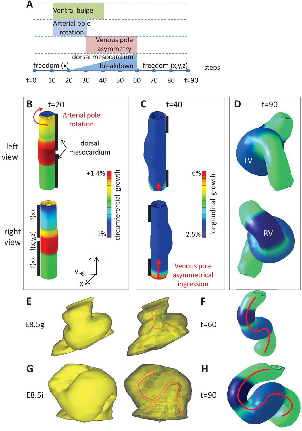
Computer simulations of heart looping integrating mechanical constraints and left-right asymmetries.
(A) Timeline of the simulations, with the successive events reflecting experimental observations. (B) Simulation of heart shape changes in 3D with a Finite Element model of a straight tube, seen from left (top) and right (down) views. The arterial pole asymmetry is modelled as a circumferential contraction (negative circumferential growth) on the right side and an expansion (positive circumferential growth) on the left side, both in a gradient towards the mid-length of the tube. The asymmetry at the arterial pole is calibrated to generate a 25° rotation. Simultaneously, the inflation of the ventricular chambers and the breakdown of the dorsal mesocardium (black bars), from the mid-length of the tube, are initiated. Where the dorsal mesocardium is present, the tube is free to move only along the x direction (f(x)). Where it has broken down, the tube is free to move along all the three directions (f(x,y,z)). (C) The venous pole asymmetry is modelled as a difference (2.8-fold) in longitudinal growth between the right and the left side. At this stage, breakdown of the dorsal mesocardium has progressed towards the poles, and thus, the tube is free along half of its length. (D) 3D shape of the cardiac tube at the end of the simulation showing the typical helix of the looped heart tube. The right (RV) and left (LV) ventricles are in darker and lighter blue, respectively. (E–H) Comparison of biological and simulated shapes. (E) Ventral views of 3D reconstructions of the heart tube at E8.5g, when looping begins. On the right, the myocardial layer (yellow) is made transparent, revealing the tube axis (red), and the notochord behind (green). (F) Ventral view of a simulated heart tube at step 60. The axis of the tube is shown as a red line. (G) Ventral views of 3D reconstructions of the heart tube at E8.5i, when looping has progressed to a counter-clockwise helix (as seen from the arterial pole). (H) Ventral view of a simulated heart tube at step 90.
Figure 6—figure supplement 1
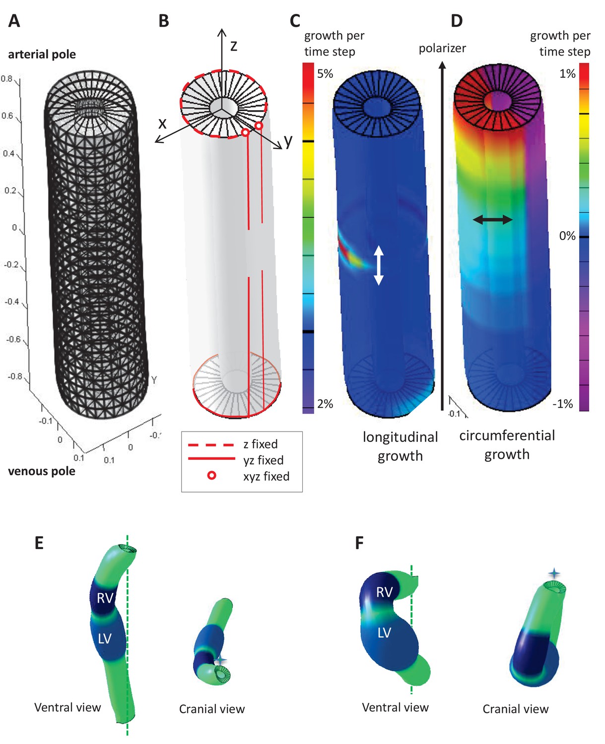
Parameters of the computer model.
(A) Hollow-cylinder model of the heart tube, made of 1800 finite elements. (B) Mechanical constraints due to the attachment of the heart tube to the rest of the body: the arterial pole extremities of the dorsal mesocardium (red circles) are used as reference points and are fixed in all three directions; the dorsal mesocardium is modelled as two parallel vertical lines (red), initially fixed along the dorsal-ventral (y) and the anterior-posterior (z) directions, and progressively released from the mid-length of the tube; the tube extremities are only constrained in z, reflecting the fact that the distance between them remains constant. (C–D) Each finite element may either grow parallel (C, longitudinal growth) or perpendicular (D, circumferential growth) to the direction defined by the gradient of a morphogen assumed to be diffusing from the venous pole towards the arterial pole (polarizer). Initially the tube bends ventrally as longitudinal growth is increased on the ventral side at mid-length (C), and it is bent rightward at the arterial pole, as circumferential growth is positive on the left side and negative (contraction) on the right side (D). (E) Computer simulation of heart looping using a variant model, when the venous pole is free to move. (F) Computer simulation of heart looping in conditions when there is no dorsal mesocardium. Simulated shapes are shown at step 90 in ventral (left) and cranial (right) views, with the right (RV) and left (LV) ventricles in darker and lighter blue respectively and the cranio-caudal axis as a green dotted line.
Figure 7
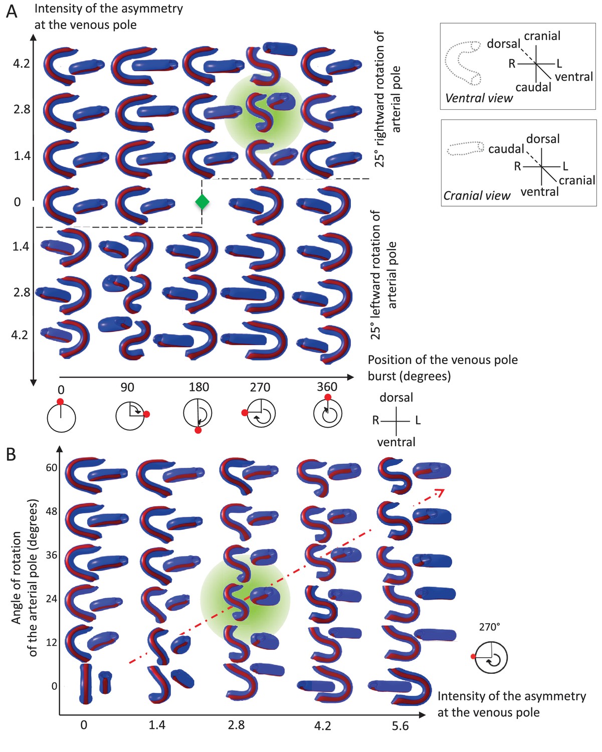
Variations in left-right asymmetries at the poles impact heart shape.
In the computer simulation, parameters of pole asymmetries were explored to analyse the variety of output shapes of the heart tube. Simulated shapes are shown at step 80 with the ventral line in red, from ventral (left) and cranial (right) views. The inflation of ventricular chambers is not simulated here. (A) In this series of simulation, the venous pole asymmetry is explored, with varying positions (abscissa) and varying intensities (ordinate). The venous pole asymmetry is simulated as a burst of growth (red dot). Its position is shown relative to the dorsal mesocardium (position 0°, with the left at 90°). The intensity of the burst is defined as a growth increase with the indicated fold difference relative to the opposite side. The angle of rotation of the arterial pole is fixed (25°), but variation in its direction is considered (rightward and leftward in the upper and lower portions of the ordinate respectively). The central green diamond indicates a centre of symmetry of the diagram. (B) In this series of simulation, the relationship between asymmetry intensities at the venous (abscissa) and arterial (ordinate) poles is explored. The venous pole asymmetry is simulated as in (A), with a fixed position (270°). The arterial pole asymmetry is simulated by a rotation of varying angle. The diagonal, which indicates proportional increase in asymmetries at the arterial and venous poles, is labelled as a red dotted arrow. The biological heart loop, which is a counter-clockwise helix (as seen in a cranial view), corresponds to a narrow window of parameter space, which is highlighted in green.
Figure 8 with 1 supplement
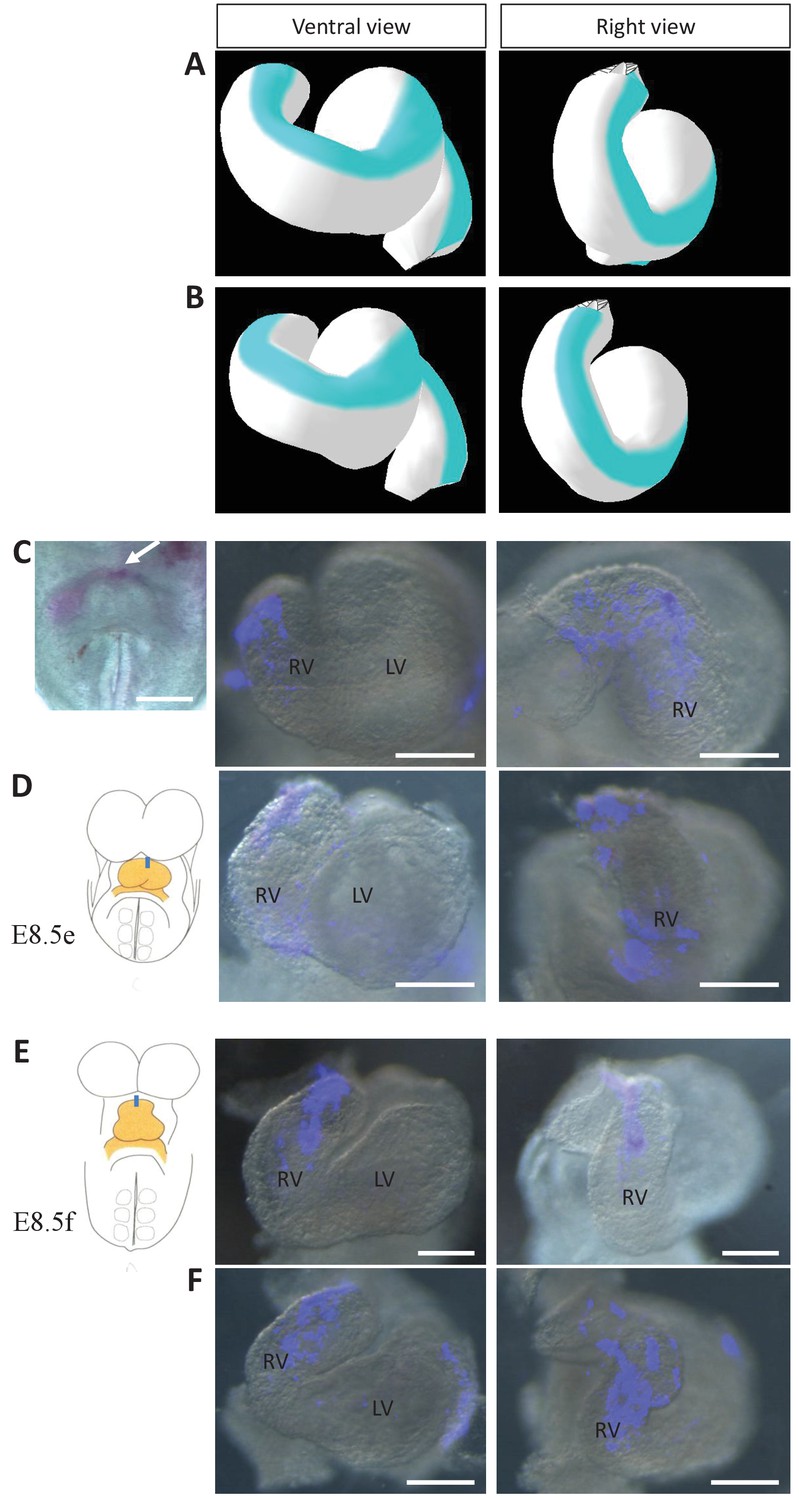
Model prediction and experimental validation of the rotation of the ventral line.
(A–B) Computer simulations of heart looping with the fate of the initial ventral line shown in blue. The simulated shape is shown at step 90 in ventral (left) and right-lateral (right) views. When the asymmetry at the arterial pole is simulated by differential longitudinal growth between the left and right, the blue line remains ventral throughout the simulation (A). When the asymmetry at the arterial pole is simulated by a rightward rotation (25°), as in Figure 6, the blue line is displaced to the right (B). (C–D) An example of a heart at E8.5e is shown on the left in C, just after DiI labelling at the most cranial ventral midline (white arrow). This is schematised on the left in D. Fluorescent signal on brightfield images of hearts, after 24 hr culture are shown on the right. The initial ventral line has been displaced to the right (n = 2/2). (E–F) Similar images of hearts, after 24 hr culture of an E8.5f embryo, labelled by DiI at the most cranial ventral midline (see scheme). The initial ventral line has been displaced to the right (n = 4/5). Scale bars: 100 µm.
Figure 8—figure supplement 1
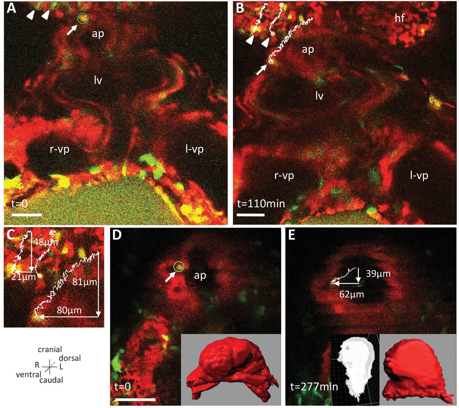
Live-imaging of the rotation of the arterial pole.
Polr2aCreERT2/+; R26Rtdtomato/YFP embryos, are shown, after injection of a low dose of tamoxifen generating fluorescent cell mosaicism. (A–B) Initial and final images of a time-lapse movie between E8.5f and E8.5g, showing the tracks of reference headfold cells (arrowheads) and a cell at the arterial pole of the heart (arrow). (C) A close-up of the cell tracks is shown, with measurements of the cranio-caudal (vertical) and lateral (horizontal) displacements. (D–E) Initial and final images of an independent time-lapse movie, between E8.5e and E8.5g, showing the track of a cell at the arterial pole of the heart (arrow). Insets are 3D projections of the heart shape, from a ventral view (red) and right lateral view (white), with the position of the tracked cell in green. ap, arterial pole; hf, headfold; L, left; LV, left ventricle; l-vp, left venous pole; R, right; r-vp, right venous pole. Scale bars: 50 μm.
Figure 9 with 3 supplements
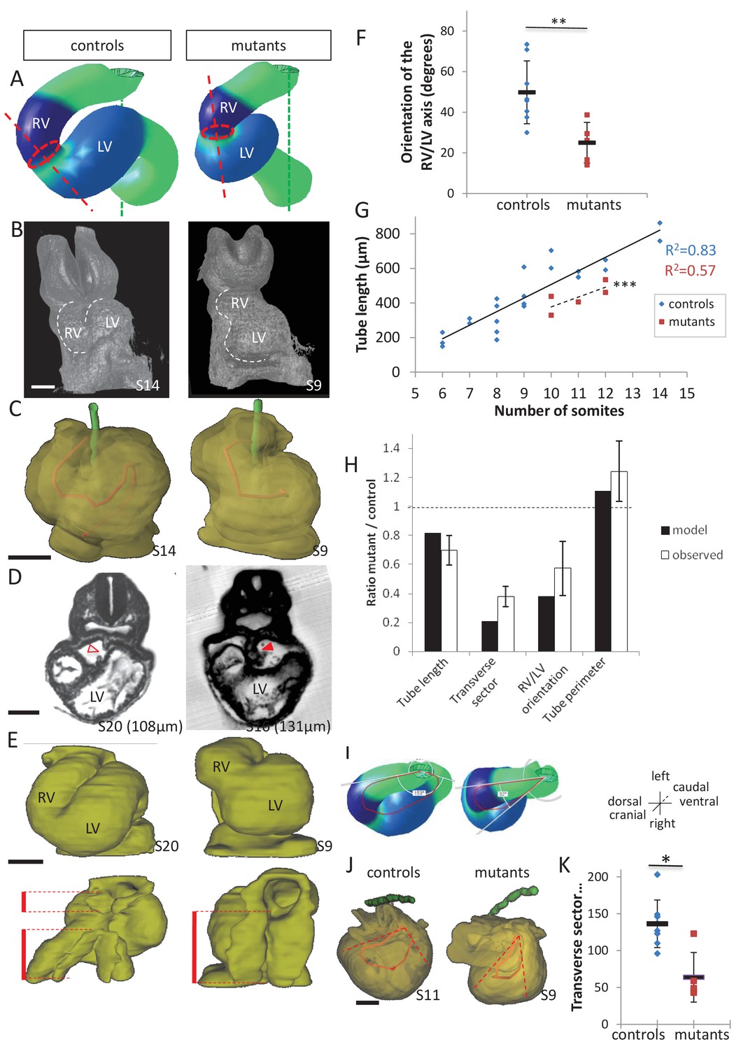
Model prediction and experimental validation, in the case of persistent dorsal mesocardium.
(A) Computer simulations of heart looping in control conditions (left), as in Figure 6, and when the dorsal mesocardium is persistent (right, simulated mutant). Simulated shapes are shown at step 90 in a ventral view, with the right (RV) and left (LV) ventricles in darker and lighter blue, respectively. The right ventricle-left ventricle axis (red dotted line) remains closer to the cranio-caudal axis (green dotted line) in the simulated mutant compared to control. (B) 3D visualisation of HREM images of a control (left) and Shh-/- mutant (right) embryo at E8.5, seen in a ventral view. (C) 3D reconstructions of the hearts shown in B, aligned with the notochord vertical (green). The axis of the myocardial tube is highlighted in red. (D) HREM section of a control embryo (left, E8.5j, 11 somites) showing the broken down dorsal mesocardium (red open arrowhead), and of a Shh-/- mutant embryo (right, 12 somites), showing persistence of the dorsal mesocardium (red arrowhead) for a myocardial tube of similar length (549 µm in the control and 535 µm in the mutant). The position of the section along the notochord is indicated in brackets. (E) 3D reconstructions from HREM images of a control (left) and a Shh-/- mutant (right) heart in ventral (top) and dorsal (bottom) views. The extent of the dorsal mesocardium is shown as a red bar on the side. (F) Graph showing the orientation of the right ventricle-left ventricle axis in control (n = 8) and Shh-/- mutants (n = 5) at 10 to 12 somite stages. (G) Graph showing the increase in the length of the myocardial tube as a function of the somite number, in control (blue) and Shh-/- mutant (red) embryos. The least-square linear regression lines and the Pearson coefficient R2 are shown for both the controls (continuous line, n = 22) and mutants (dotted line, n = 5). The two slopes are not significantly different, but the y-intercepts are (ANCOVA, p-value=0.001), indicating that the mutants have a significantly shorter tube length. (H) Validation of quantitative predictions raised by computer simulations for four geometrical parameters. (I) Cranial views of simulated hearts (left, control, right, mutant), showing the tube axis in red and the transverse sector in which it is inscribed in white. (J) 3D reconstructions from HREM images of a control (left) and Shh-/- mutant (right) heart, shown in a cranial view. The axis of the myocardial tube is in red, and the transverse sector in which it is inscribed is shown as red dotted lines. (K) Quantification of the angles of these transverse sectors in controls (blue, n = 8) and Shh-/- mutants (red, n = 5). The heart tube helix is significantly wider in control samples (*p-value<0.05, Mann-Whitney U test). Means and standard deviations are shown. Scale bars: 100 µm.
-
Figure 9—source data 1
3D reconstructions of all hearts of Shh-/- mutants and control littermates analysed at E8.5.
Ventral (left) and dorsal (right) views are shown, aligned with the notochord vertical (green). The myocardial layer (yellow) is made transparent, revealing the tube axis (red). Samples are identified with a number (S). The length of the heart tube is indicated, as well as the somite number (So) of the corresponding embryo. The genotype of control samples is Shh+/+ (S11, S17, S20) or Shh+/- (S8, S14). Scale bar: 100 µm.
- https://doi.org/10.7554/eLife.28951.022
Figure 9—figure supplement 1
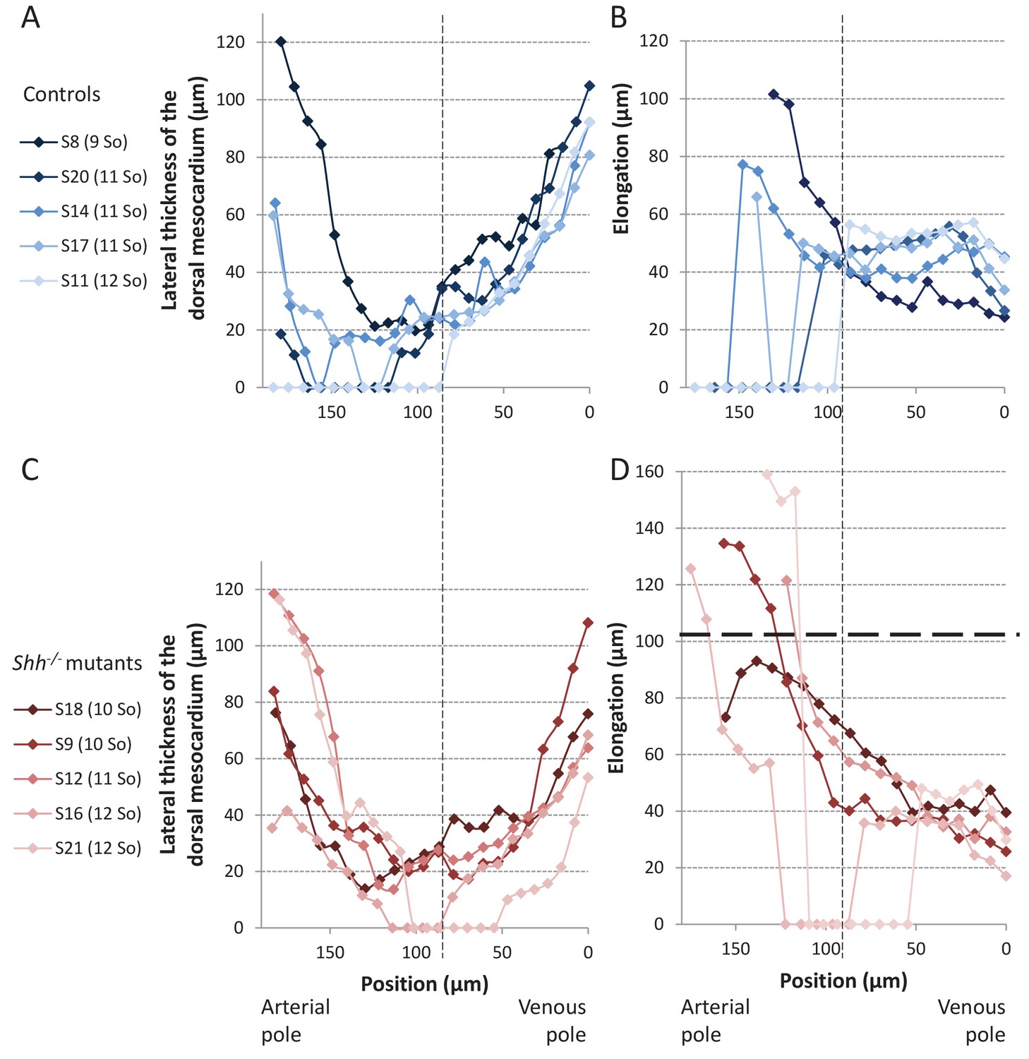
Structure of the dorsal mesocardium in Shh-/- mutants and control littermates at E8.5.
(A, C) Lateral thickness of the dorsal mesocardium, measured as in Figure 3D, in five controls (A) and 5 Shh-/- mutant hearts (C) at E8.5. Samples are identified with a number (S), and the somite number (So) of the embryo is indicated in brackets. The boundary between the arterial and venous halves of the tube is shown by a vertical dashed line. (B, D) Ventral elongation of the dorsal mesocardium, measured as in Figure 3F, in the same controls (B) and Shh-/- mutant hearts (D). The maximum value observed in controls is shown with an horizontal thick dashed line.
Figure 9—figure supplement 2
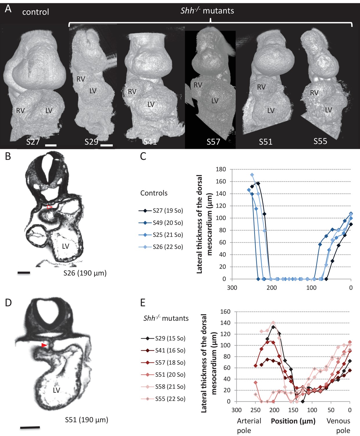
Shh-/- mutants and control littermates at E9.5.
(A) 3D visualisation of HREM images of a control (left) and Shh-/- mutant (right) embryos, seen in a ventral view. The presence of the pericardium (S55) provides a rough appearance to the heart. (B, D) HREM section of a control embryo (B) showing the broken down dorsal mesocardium (red open arrowhead), and of a Shh-/- mutant embryo (D), showing persistence of the dorsal mesocardium (red arrowhead). Samples are identified with a number (S), and the position of the section is indicated in brackets. (C, E) Lateral thickness of the dorsal mesocardium, measured as in Figure 3D, in four controls (C) and 6 Shh-/- mutants (E). The somite number (So) of embryos is indicated in brackets. Scale bars: 100 µm.
Figure 9—figure supplement 3
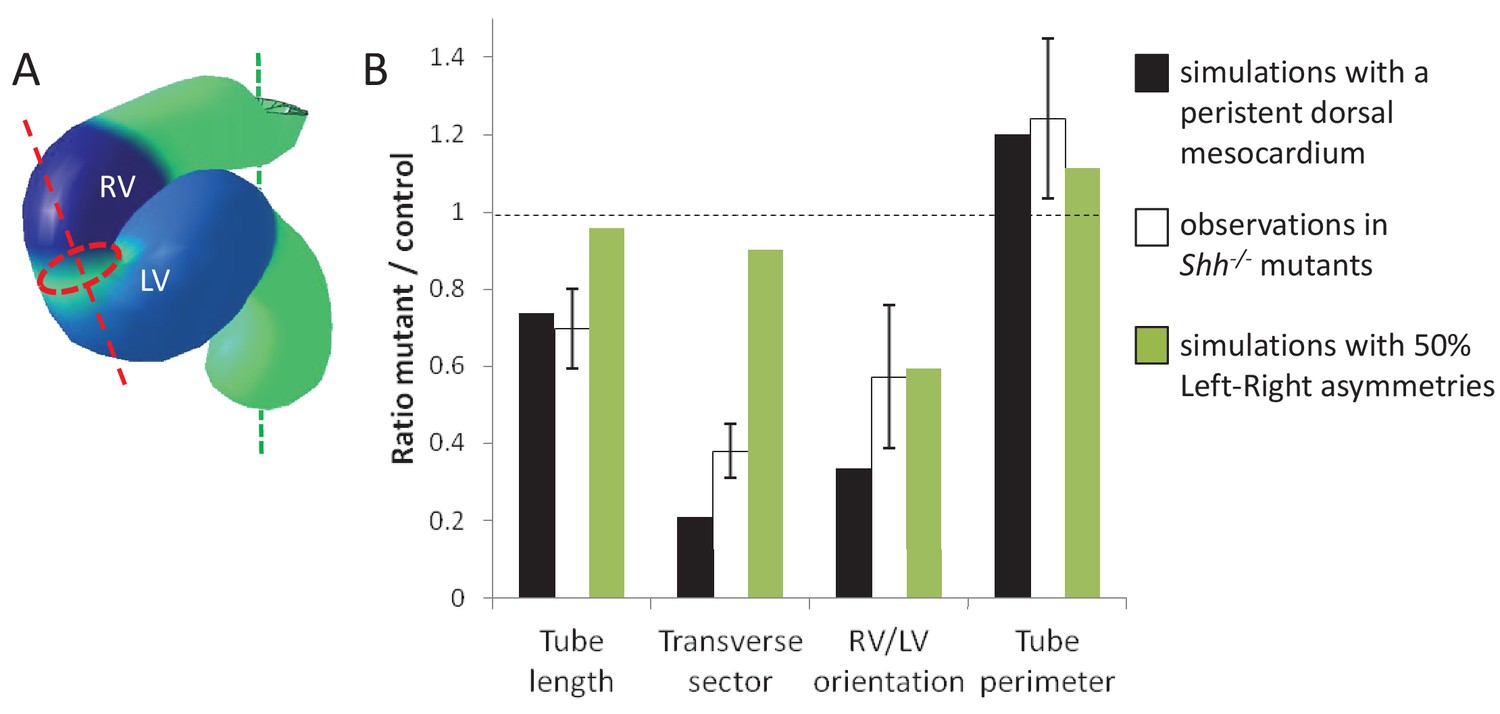
Alternative simulations and comparison with Shh-/- mutant hearts.
Comparison between quantitative predictions for four geometrical parameters raised by two types of computer simulations and biological measures in Shh-/-mutant hearts at E8.5. Simulation with 50% left-right asymmetries correspond to a 12° rotation at the arterial pole and a 1.4-fold asymmetric ingression at the venous pole.
Figure 10
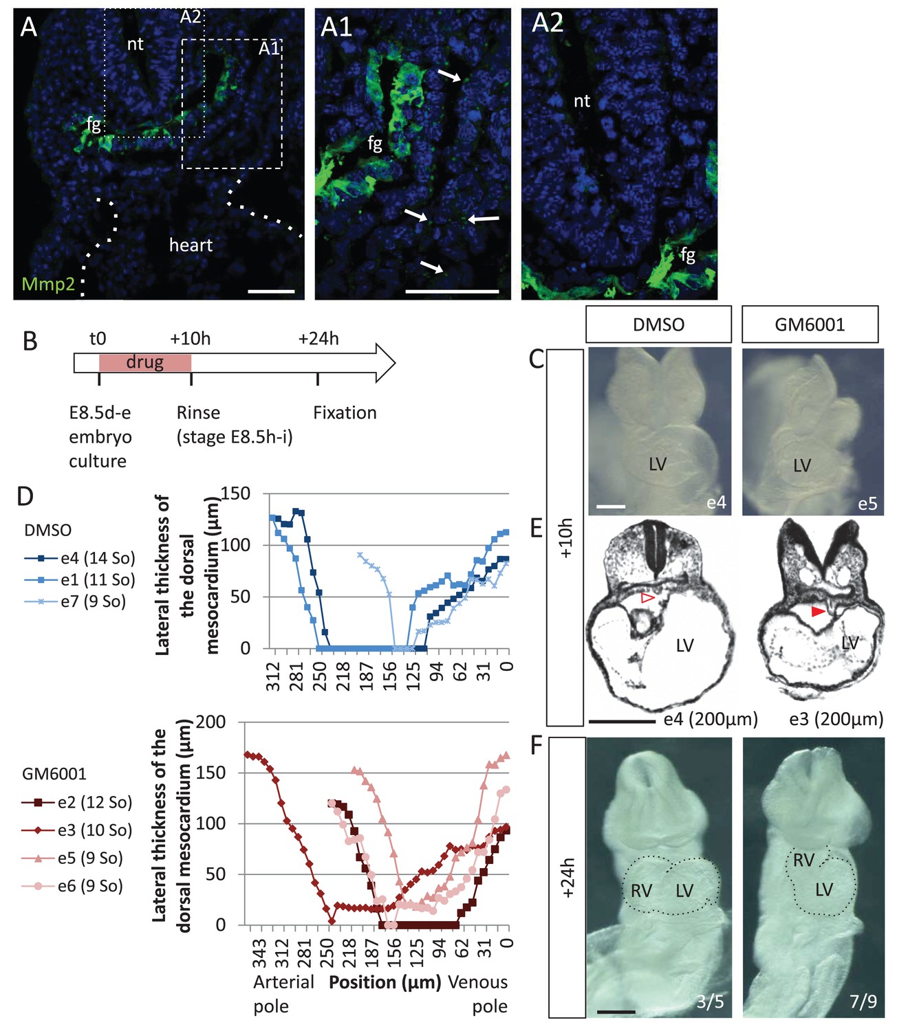
Matrix metalloproteases are required for dorsal mesocardium breakdown and heart looping.
(A) Immunostaining of Mmp2, showing expression in the foregut (fg) at E8.5g, and vesicular localisations in the cardiac region (arrowheads in A1), but not in the neural tube (nt, A2). Maximum intensity projections are shown, over 14 (A), 35 (A1) or 31 (A2) z-sections. (B) Scheme of the experimental procedure. (C) Brightfield images of embryos after 10-hr culture with GM6001, an inhibitor of matrix metalloproteases, or the adjuvant (DMSO). (D) Quantification of the lateral thickness of the dorsal mesocardium, measured as in Figure 3D, in 3 DMSO (up) and 4 GM6001 (down) treated embryos after 10 hr of culture. Samples are identified with a number (e), and the somite number (So) of the embryo is indicated in brackets. (E) HREM sections of embryos showing a broken down dorsal mesocardium (red open arrowhead) upon DMSO treatment, and a persistent dorsal mesocardium (red arrowhead) upon GM6001 treatment. The position of the section along the notochord is indicated in brackets. (F) Brightfield images of embryos after 24 hr culture. The frequency of normal looping, in the presence of DMSO, or abnormal heart looping, in the presence of GM6001, is indicated in the lower right corner. The contour of the heart tube is outlined. LV, left ventricle; RV, right ventricle. Scale bars: 50 µm (A), 200 µm (C, E–F).
Videos
Video 1
Example of a 3D stack of HREM images acquired from an embryo at E8.5h.
Video showing the successive sections of an E8.5h embryo, at the level of the heart. Images were acquired by HREM every 2 µm.
Video 2
Computer simulation of heart looping in the control situation.
https://doi.org/10.7554/eLife.28951.013
Video 3
Example of live-imaging of the arterial pole rotation.
Video related to Figure 8—figure supplement 1A–C.
Video 4
Computer simulation of heart looping in the case of persistent dorsal mesocardium.
https://doi.org/10.7554/eLife.28951.023Tables
Key resources table
| Reagent type (species) or resource | Designation | Source or reference | Identifiers | Additional information |
|---|---|---|---|---|
| Strain, strain background (Mus musculus) | wild-type, Swiss background | Janvier | ||
| Strain, strain background (Mus musculus) | wild-type, C57Bl6 background | Janvier | ||
| Strain, strain background (Mus musculus) | T4nLacZ, Swiss background | Biben et al. (1996) doi:10.1006/dbio.1996.0017 | PMID 8575622 | |
| strain, strain background (Mus musculus) | Shh+/-, C57Bl6J background | Gonzalez-Reyes et al. (2012) doi:10.1016/j.neuron.2012.05.018 | MGI:5440762 | |
| Strain, strain background (Mus musculus) | Polr2aCreERT2/+, C57Bl6 background | Guerra et al. (2003) PMID:12957286 | MGI:3772332 | |
| Strain, strain background (Mus musculus) | R26YFP/+, C57Bl6 background | Srinivas et al. (2001) PMID:11299042 | MGI:2449038 | |
| Strain, strain background (Mus musculus) | R26Rtdtomato/+ (Ai14), C57Bl6 background | Madisen et al. (2010) doi:10.1038/nn.2467 | MGI:3809524 | |
| Antibody | anti-PH3 (rabbit monoclonal) | Abcam | Abcam: ab32107 | (1:100) |
| Antibody | anti-Isl1 (mouse monoclonal) | Developmental Studies Hybridoma Bank | DSHB: 39.4D5 | (1:50) |
| Antibody | anti-MMP2 (mouse monoclonal) | Santa Cruz | Santa Cuz: sc13594 | (1:50) |
| Antibody | goat anti-rabbit IgG Alexa Fluor 546 | Invitrogen | Invitrogen: A11035 | (1:500) |
| Antibody | goat anti-mouse IgG2b Alexa Fluor 488 | Invitrogen | Invitrogen: A21141 | (1:500) |
| Antibody | goat anti-mouse IgG1 Alexa Fluor 488 | Invitrogen | Invitrogen: A21121 | (1:500) |
| Commercial assay or kit | JB-4 embedding kit | Polysciences | Polysciences: 00226–1 | |
| Chemical compound, drug | GM6001 (Ilomast) | Millipore | Millipore: CC1000 | 10 µM |
| Software, algorithm | Gftbox | Kennaway et al. (2011) doi:10.1371/journal.pcbi.1002071 | Matlab Finite Element Analysis package simulating biological growth | |
| Software | ICY | de Chaumont et al. 2012 doi:10.1038/nmeth.2075 | Open platform for bioimage informatics |
Additional files
-
Source code 1
Code used to generate Figure 2F–G.
- https://doi.org/10.7554/eLife.28951.025
-
Source code 2
- https://doi.org/10.7554/eLife.28951.026
-
Source code 3
Code used to generate Figure 7.
- https://doi.org/10.7554/eLife.28951.027
-
Source code 4
Code used to generate Figure 8A.
- https://doi.org/10.7554/eLife.28951.028
-
Source code 5
- https://doi.org/10.7554/eLife.28951.029
-
Transparent reporting form
- https://doi.org/10.7554/eLife.28951.030
Download links
A two-part list of links to download the article, or parts of the article, in various formats.
Downloads (link to download the article as PDF)
Open citations (links to open the citations from this article in various online reference manager services)
Cite this article (links to download the citations from this article in formats compatible with various reference manager tools)
A predictive model of asymmetric morphogenesis from 3D reconstructions of mouse heart looping dynamics
eLife 6:e28951.
https://doi.org/10.7554/eLife.28951


