Magnetic eye tracking in mice
- Stanford University, United States
Figures
Figure 1 with 1 supplement
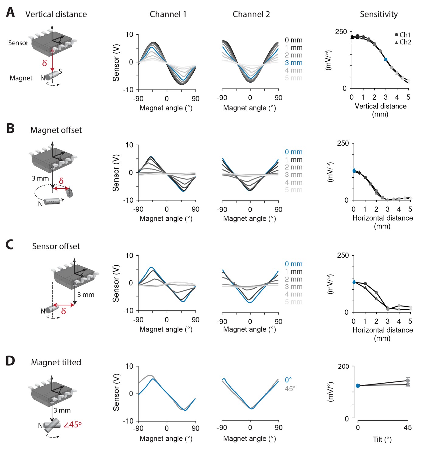
Systematic testing of magnet-sensor placement.
(A) Output of the magnetic sensor when a 0.75 × 2 mm cylinder magnet was rotated by a servo-controlled motor. Left, Schematic showing the relative position and orientation of the magnet and sensor, the axis of magnet rotation (dashed line and arrow) and the dimension along which magnet position was varied (δ, red arrow). Middle, Output from each channel of the magnetic sensor as vertical distance (δ) between the magnet and the surface of the sensor was varied from 0 mm (black) to 5 mm (light grey) (n = 5 repeated measurements). Right, Sensitivity of each channel of the magnetic sensor at each distance from the magnet. In this and all panels, SEM for repeated measurements was smaller than the symbol size. (B) Same as in (A), but the magnet was offset horizontally (δ) from both its axis of rotation and the center of the sensor. Vertical distance was fixed at 3 mm. (C) Same as in (B), but the sensor was offset horizontally from the center of the magnet, which rotated about its center. (D) Same as in (B), but comparing horizontal orientation of the magnet as in (A) with a 45° tilt relative to the plane of the sensor (p=0.168, n = 5 repeated measurements, two sample t-test). Vertical distance between the center of the magnet and the sensor was fixed at 3 mm.
Figure 1—figure supplement 1
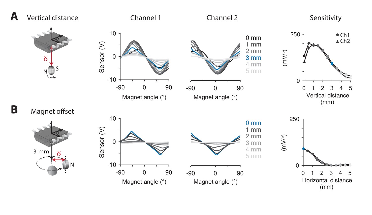
Systematic testing of magnet-sensor placement for a disc magnet.
(A) Output of the magnetic sensor when a 1.5 × 0.5 mm disc magnet was rotated by a servo-controlled motor. Left, schematic of magnet-sensor orientation. Middle, output from each channel of the magnetic sensor as the vertical distance (δ) between the magnet and the surface of the sensor was varied from 0 mm (black) to 5 mm (light grey) (n = 5 repeated measurements). Right, sensitivity of each channel of the magnetic sensor at each distance from the magnet. (B) Same as in (A), but the magnet was horizontally offset (δ) from both its axis of rotation and the center of the sensor.
Figure 2
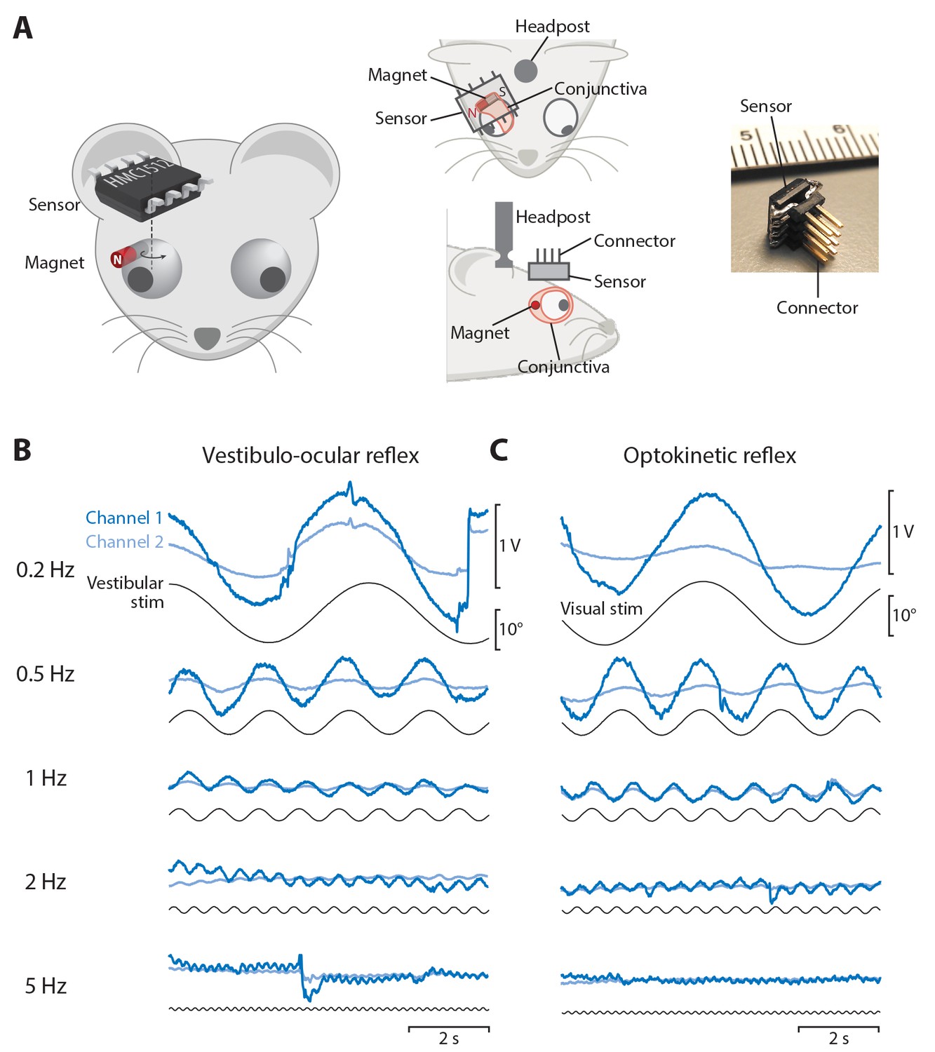
Magnetic eye tracking in mice.
(A) Schematic of the magnetic eye tracking system, illustrating the orientation of the sensor relative to the magnet and eye. The magnet was implanted beneath the conjunctiva on the temporal side of the eye. The sensor was soldered to an 8-pin connector and positioned over the magnet in a plane parallel to that of horizontal (nasal-temporal) eye movements. An implanted head post was used to restrain the head so that the nasal-temporal axis of the eye was earth-horizontal. (B) Raw output from both channels of the magnetic sensor (blue traces) during the vestibulo-ocular reflex (VOR) in one example mouse. A vestibular stimulus (black trace, head position) was delivered by rotating the animal about an earth-vertical axis in the dark (0.2 Hz to 5 Hz, peak velocity ±10°/s). (C) Raw output from the magnetic sensor during the optokinetic response (OKR). A visual stimulus (black trace) was delivered by rotating a vertically striped drum, which surrounded the mouse, about an earth-vertical axis (0.2 Hz to 5 Hz, peak velocity ±10°/s).
Figure 3
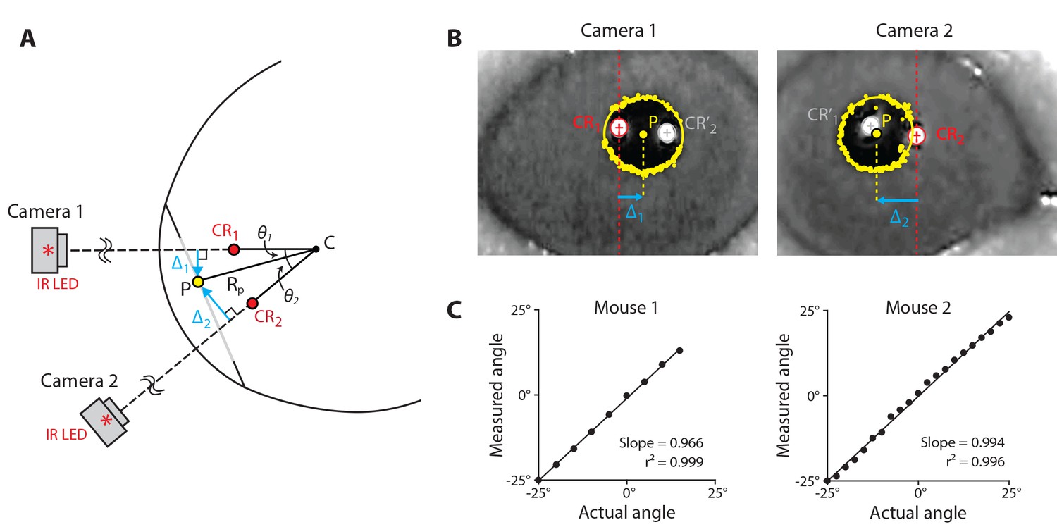
Dual-angle video-oculography.
(A) Schematic of the eye as viewed from above, illustrating the dual-angle video-oculography technique. Two cameras were affixed to a platform, with their axes at an angle of 40° relative to each other, and with the cameras equidistant (5 cm) from the point at which their axes intersected. An infrared LED mounted directly above each camera created a corneal reflection (CR). The position of the camera platform was adjusted to align the image of each CR to the center of the corresponding camera’s image (CR1, CR2; red). This aligned both camera axes with the center of corneal curvature (C), and ensured that the two cameras were equidistant from the eye, and therefore had the same image magnification. The distances ∆1 and ∆2 from the CR to the center of the pupil (P) in each camera’s image were used to compute the angular position of the pupil relative to the cameras (θ1, θ2) (see Materials and methods, Equation 9). (B) Example camera frames showing the software-detected pupil and CR locations for each camera. CR1ʹ and CR2ʹ (grey) are reflections generated by the infrared LED above the opposite camera, and are ignored. Other abbreviations as in (A). (C) Validation of dual-angle video-oculography. Eye position measured by using video-oculography is plotted against true angle as the camera system was rotated about the eye of two anesthetized mice.
Figure 4
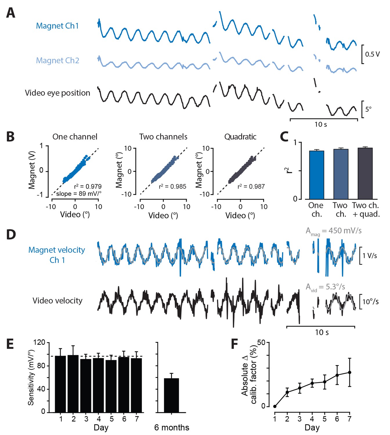
Calibration of magnetic eye tracking using video-oculography.
(A) Simultaneously recorded magnetic sensor output (Ch1 dark blue, Ch2 light blue) and video-derived eye position (black) from one example mouse, measured during vestibular stimulation in the light. (B) Signals from the magnetic sensor, compared time point-by-time point against eye position measured by video-oculography, for the example mouse in (A). Results are shown for models of increasing complexity, from left to right: inputs to the regression model included the single best magnetic sensor channel alone (‘One channel’), both magnetic sensor channels (‘Two channels’), or two channels plus quadratic terms (‘Quadratic’) (see Materials and methods). (C) Mean correlation coefficients between video and calibrated magnet output for each model (n = 24 mice). (D) Calibration of magnetic sensor using eye velocity. Example differentiated video and magnetic sensor traces are shown for same mouse as in (A). The sine wave fit to the magnetic sensor channel with higher r2 relative to the video is shown. The output of the magnetic sensor channel was scaled by a calibration factor equal to the ratio of video sine wave amplitude (Avid) divided by magnetic sensor amplitude (Amag). (E) Stability of magnetic eye tracking over time. Sensitivity was quantified as the reciprocal of the calibration factor obtained using the velocity method, and was measured each day for one week, and six months after magnet implantation. Mean sensitivity did not change over one week (all p>0.3, paired t-test, Days 2–7 vs. Day 1, n = 8). After six months (average time post-surgery 6.0 ± 0.4 months, range 5.2–7.7 months), sensitivity was lower but still robust (n = 8 mice; two additional mice had no detectable eye movement signals). (F) Changes in the calibration factor of individual mice over time. Although the mean sensitivity of the magnetic sensor was robust over months, the calibration factors of individual mice showed some fluctuations from day-to-day, as quantified by the absolute value of the percent change in calibration factor measured each day for one week, relative to Day 1.
Figure 5
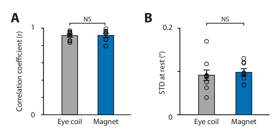
Comparison of magnetic eye tracking with the eye coil technique.
(A) Correlation coefficient between the video and the eye coil data (gray; symbols represent individual mice, n = 9) and between the video and magnetic eye tracking data (blue, n = 8 mice) (p=0.937; two-sample t-test for eye coil vs. magnet). (B) Spatial resolution was similar for the eye coil and magnetic eye tracking systems (p=0.631, two-sample t-test), as measured by the standard deviation of eye position signals recorded during epochs when the eyes were relatively stationary in head-fixed mice in the light.
Figure 6 with 2 supplements

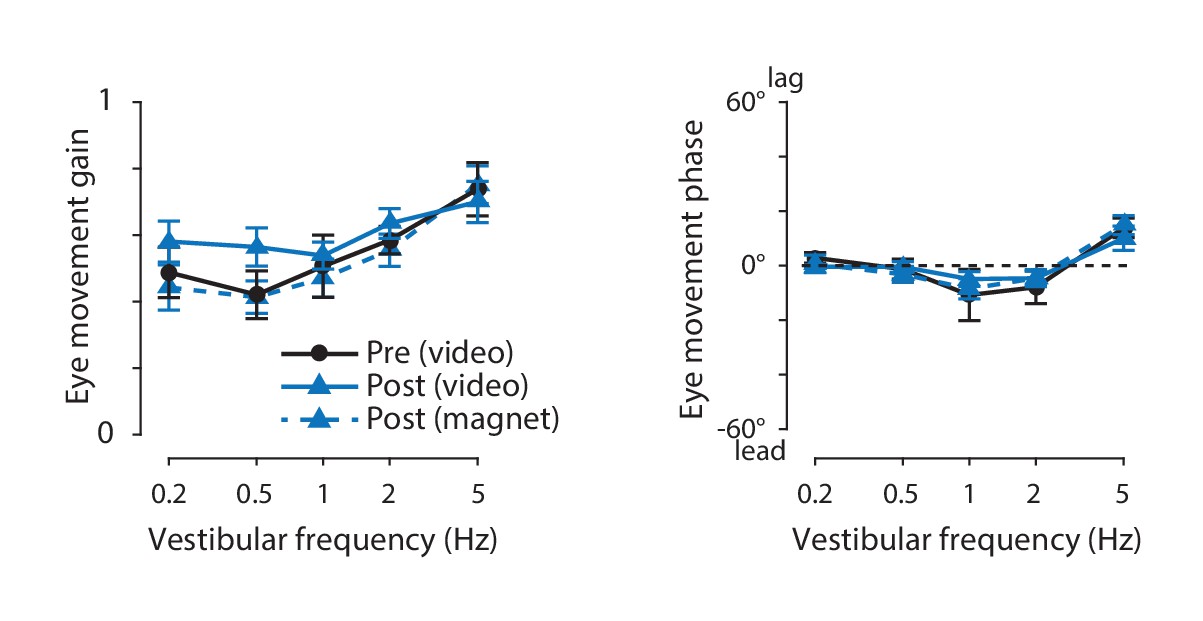
The vestibulo-ocular reflex (VOR) before and after magnet implantation.
The gain (left) and phase (right) of the eye movement responses to vestibular stimuli, before (black) and six days after (blue) implantation of the magnet and sensor, measured using video-oculography with infrared illumination in otherwise complete darkness (solid lines). There was no effect of magnet implantation on either the gain or the phase of the VOR (p=0.725 gain, p=0.350 phase, for main effect of pre- vs post-implantation; p=0.497 gain, p=0.469 phase, for interaction with vestibular stimulus frequency; two-way repeated measures ANOVA, n = 8 mice). The gain and phase of the VOR measured simultaneously with magnetic eye tracking (post-implantation) are shown as well (blue, dashed lines).
Figure 6—figure supplement 1
Eye movements driven by combined vestibular and visual input, before and after magnet implantation.
The gain (left) and phase (right) of the eye movement responses to the combined vestibular and visual input provided by head rotations in an illuminated visual surround was measured using video-oculography (solid lines) before (black) and after (black) implantation of the magnet and sensor. There was no effect of magnet implantation on either the gain or the phase of the eye movements (p=0.447 gain, p=0.794 phase, for main effect of pre- vs post-implantation; p=0.618 gain, p=0.488 phase, for interaction with vestibular stimulus frequency; two-way repeated measures ANOVA, n = 8 mice). The gain and phase of the eye movements measured simultaneously with magnetic eye tracking (post-implantation) are shown also (blue, dashed lines). The visual input included both a mouse-stationary video apparatus, which would tend to suppress the eye movements driven by the vestibular stimulus, and an earth-stationary visual surround, which would tend to enhance the eye movements driven by the vestibular stimulus.
Figure 6—figure supplement 2
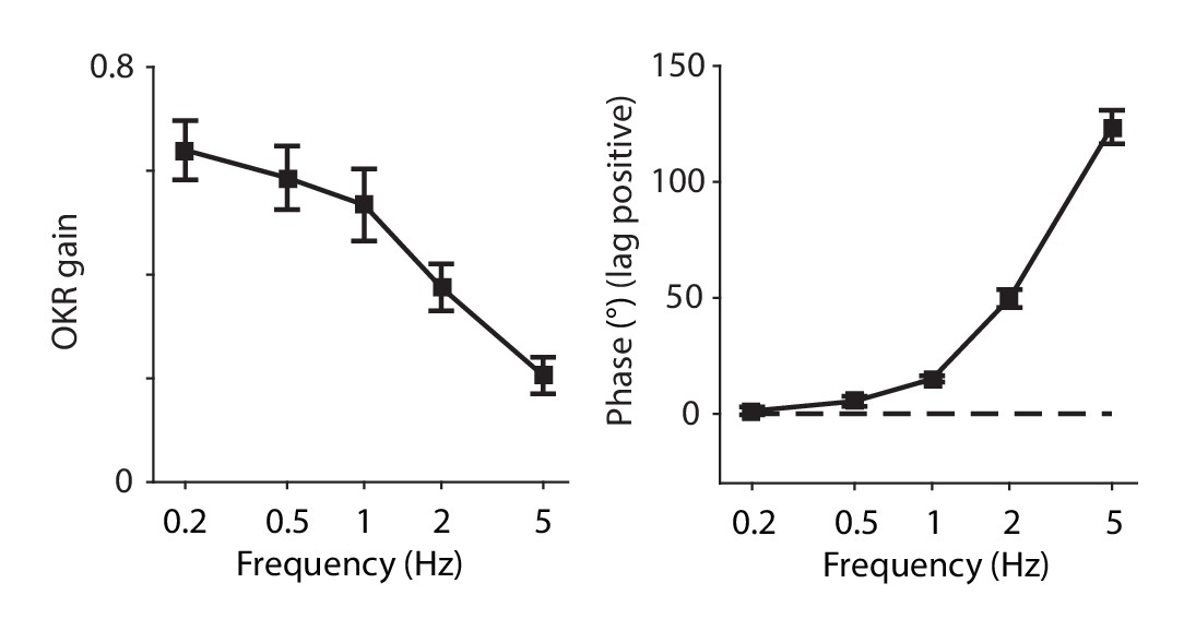
The optokinetic response (OKR) measured with magnetic eye tracking.
The gain (left) and phase (right) of the OKR elicited by rotation of a random checkerboard patterned drum around the mouse, measured using the magnetic eye tracking system (n = 6 mice).
Figure 7
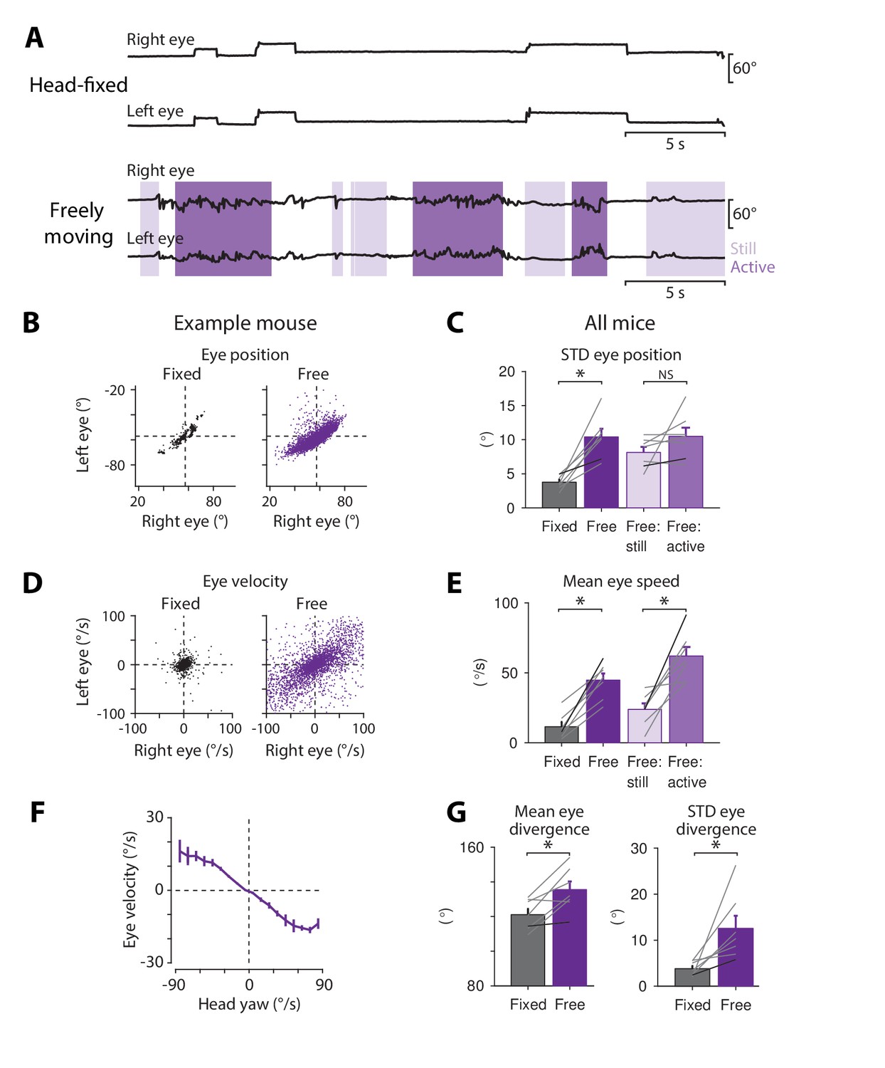
Eye movements measured in freely moving mice.
(A) Example of bilateral eye movements in one mouse when it was head-fixed (top) compared to freely moving (bottom). Light purple, body still; dark purple, body actively moving, as measured using overhead video images (see Materials and methods). (B) Scatterplot of left and right eye positions in the example mouse from (A), during head fixation (black, left) and during free motion (purple, right). (C) Variability of eye position in head-fixed and freely moving mice. The standard deviation of eye position increased in head-free (dark purple) compared with head-fixed (black) mice (p=1.9 × 10⁻⁴, paired t-test, n = 7). Eye movements recorded in head-free mice were further subdivided into periods when the body was still (light purple) versus actively moving (medium purple) (p=0.146, paired t-test, n = 7). Grey lines, individual mice; black lines, example mouse in (A). (D) Scatterplots of velocity of the left and right eye during head fixation and free motion, for the example mouse in (A). (E) Mean eye speed was higher in freely moving than head-fixed mice (p=9.7 × 10⁻⁵, paired t-test, n = 7). In unrestrained mice, eye speed was highest during periods of active body movement compared to periods when the body was relatively still (p=3.6 × 10⁻⁴, paired t-test, n = 7). (F) Correlation between horizontal eye velocity and head velocity about the yaw axis in freely moving mice (n = 4). (G) Binocular coordination in head-fixed and freely moving mice. Left, mean eye divergence (horizontal angle between the two eyes) increased during free motion compared to head fixation (p=0.029, paired t-test, n = 7). Right, the standard deviation of eye divergence also increased during free motion (p=0.009, paired t-test, n = 7).
Additional files
-
Transparent reporting form
- https://doi.org/10.7554/eLife.29222.012
Download links
A two-part list of links to download the article, or parts of the article, in various formats.
Downloads (link to download the article as PDF)
Open citations (links to open the citations from this article in various online reference manager services)
Cite this article (links to download the citations from this article in formats compatible with various reference manager tools)
Magnetic eye tracking in mice
eLife 6:e29222.
https://doi.org/10.7554/eLife.29222


