Cortical response states for enhanced sensory discrimination
- McGovern Medical School, University of Texas, United States
- Janelia Research Campus, Howard Hughes Medical Institute, United States
- Universidad de Buenos Aires, South America
Figures
Figure 1 with 4 supplements
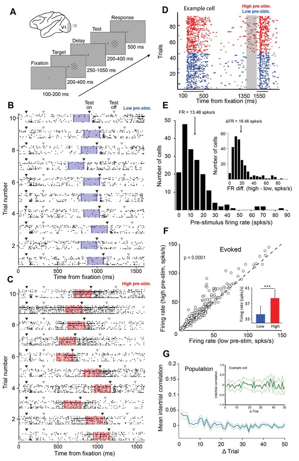
Examining the impact of cortical response state on V1 responses.
(A) Schematic representation of the experimental setup. Monkeys were trained to discriminate the orientation of lines by signaling whether two successive gratings (target and test) had the same or different orientation. If the two gratings had the same orientation, the monkey was required to release the bar within 500 ms of the offset of the test stimulus. If the target and test stimuli had different orientations, the monkey was required to continue holding the bar (the number of match and non-match stimuli was identical). (B–C) Ten example trials of 18 simultaneously recorded neurons exhibiting low (panel B) or high (panel C) firing activity before test stimulus presentation. Black arrowheads represent stimulus onset and gray arrowheads represent stimulus offset. The blue (panel B) and red (panel C) shaded regions represent the 200 ms interval before test stimulus presentation. (D) Neuronal activity during the delayed-match-to-sample orientation discrimination task. The gray shaded area indicates the interval used to classify trials into low and high pre-stimulus state trials. The colored dots represent the timing of action potentials of an example neuron in the low (blue) and high pre-stimulus trials (red). (E) Population histogram of pre-stimulus firing rates measured 200 ms before the presentation of the test stimulus. The mean pre-stimulus rate was 13.48 ± 0.86 spks/s. (Inset) histogram of firing rate change between the two pre-stimulus states. The median change in firing rate between the two states was 18.46 ± 1.04 spks/s (arrow marks bin). (F) Evoked firing rate in the high pre-stimulus response state plotted as a function of the evoked firing rate in the low pre-stimulus state (each circle corresponds to one cell). Evoked firing rate was significantly greater in the high pre-stimulus state (p<0.0001, paired t-test). (G) Mean correlation in pre-stimulus firing rates between trials for the entire population of cells (correlation values are near chance level). Error bars represent SEM. (inset) Auto-correlation of pre-stimulus firing rates for one example cell showing no significant correlation in trial-by-trial pre-stimulus firing rates (green shadow represents the 95% confidence intervals).
Figure 1—figure supplement 1
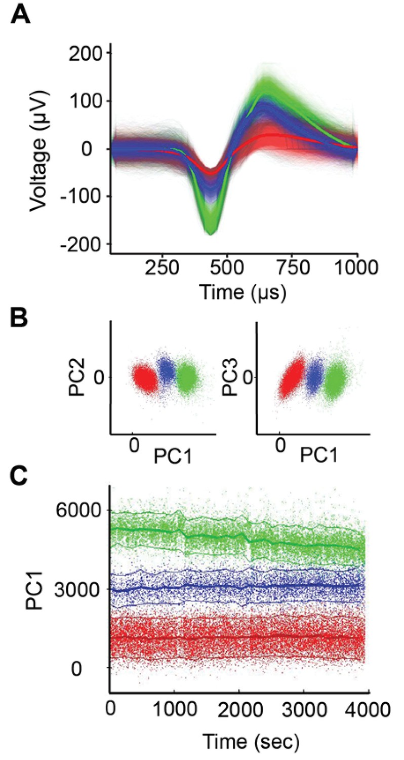
Spike sorting example.
(A) Example of single-unit spike-sorting in one session with the U-probe. There were three distinct spike waveforms isolated from the same electrode. (B) Clustering of the three units from panel A in principal component analysis (PCA) space. (C) Amplitude of PC1 as a function of time for the three units. Notice that the green cell decreases its amplitude in time, but without overlapping with the other units.
Figure 1—figure supplement 2
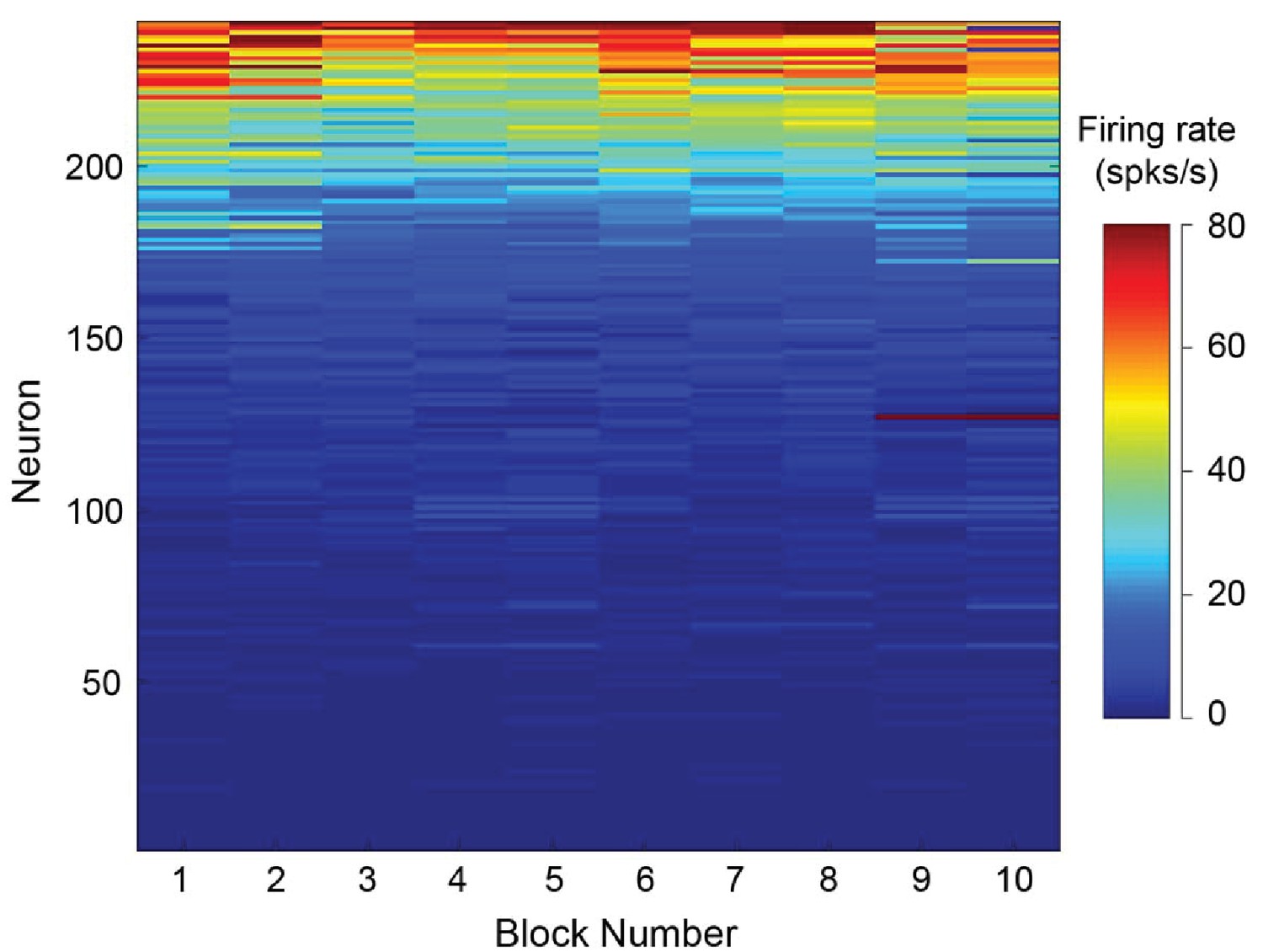
Neural stability over the recording session.
After dividing each session into ten blocks, we calculated the mean firing rate during the delay period. We observed that 99% of cells exhibited stable firing rates throughout the recording session (p>0.05, Pearson correlation of each neuron over the ten trial blocks).
Figure 1—figure supplement 3
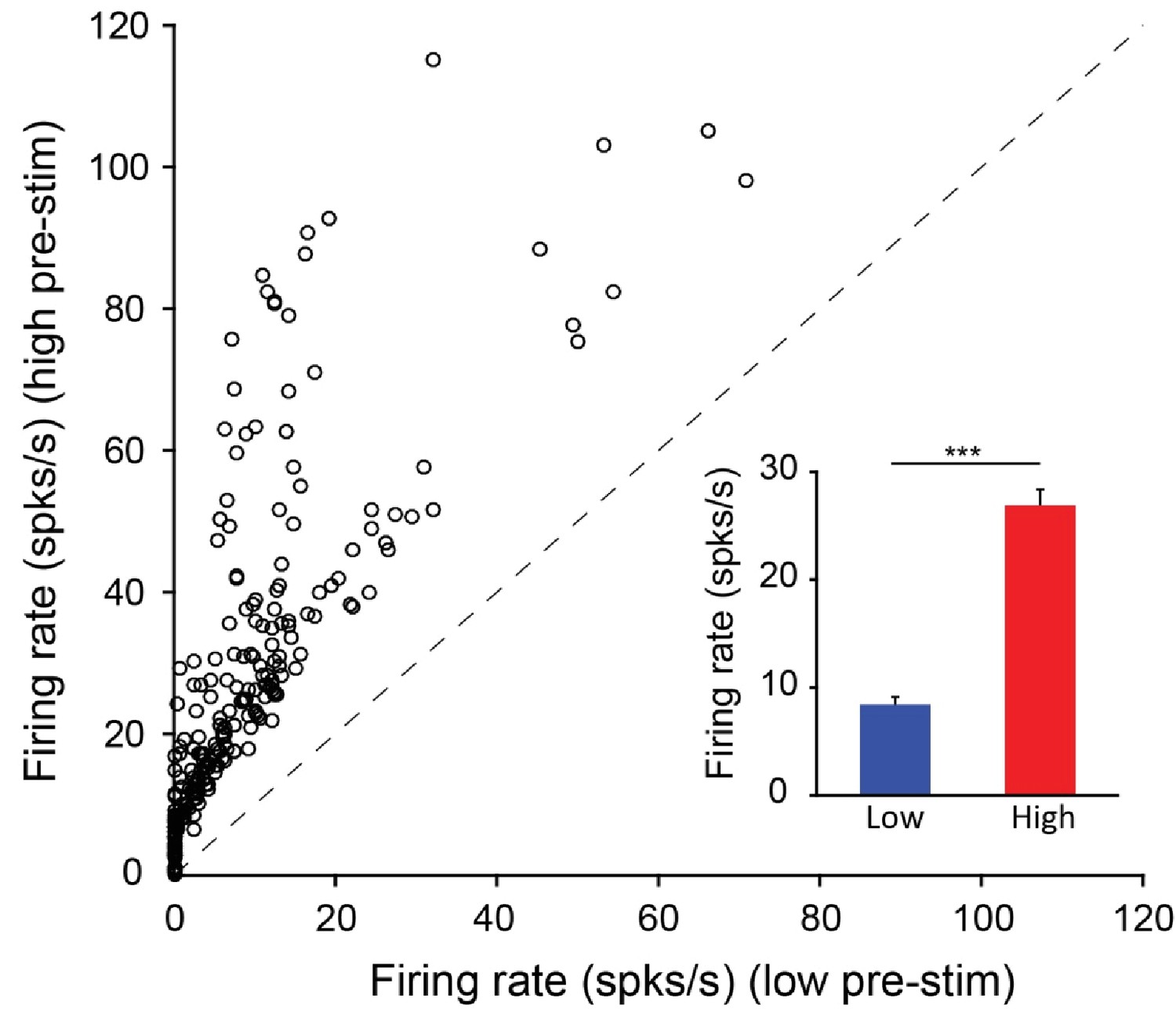
Distribution of mean firing rates in the low and high pre-stimulus periods for all the neurons recorded in the behavioral experiments.
(A) Mean firing rate in the high pre-stimulus state plotted as a function of the mean firing rate in the low pre-stimulus state. (inset) Mean firing rate for low and high pre-stimulus conditions (p<0.0001, Paired t-test).
Figure 1—figure supplement 4
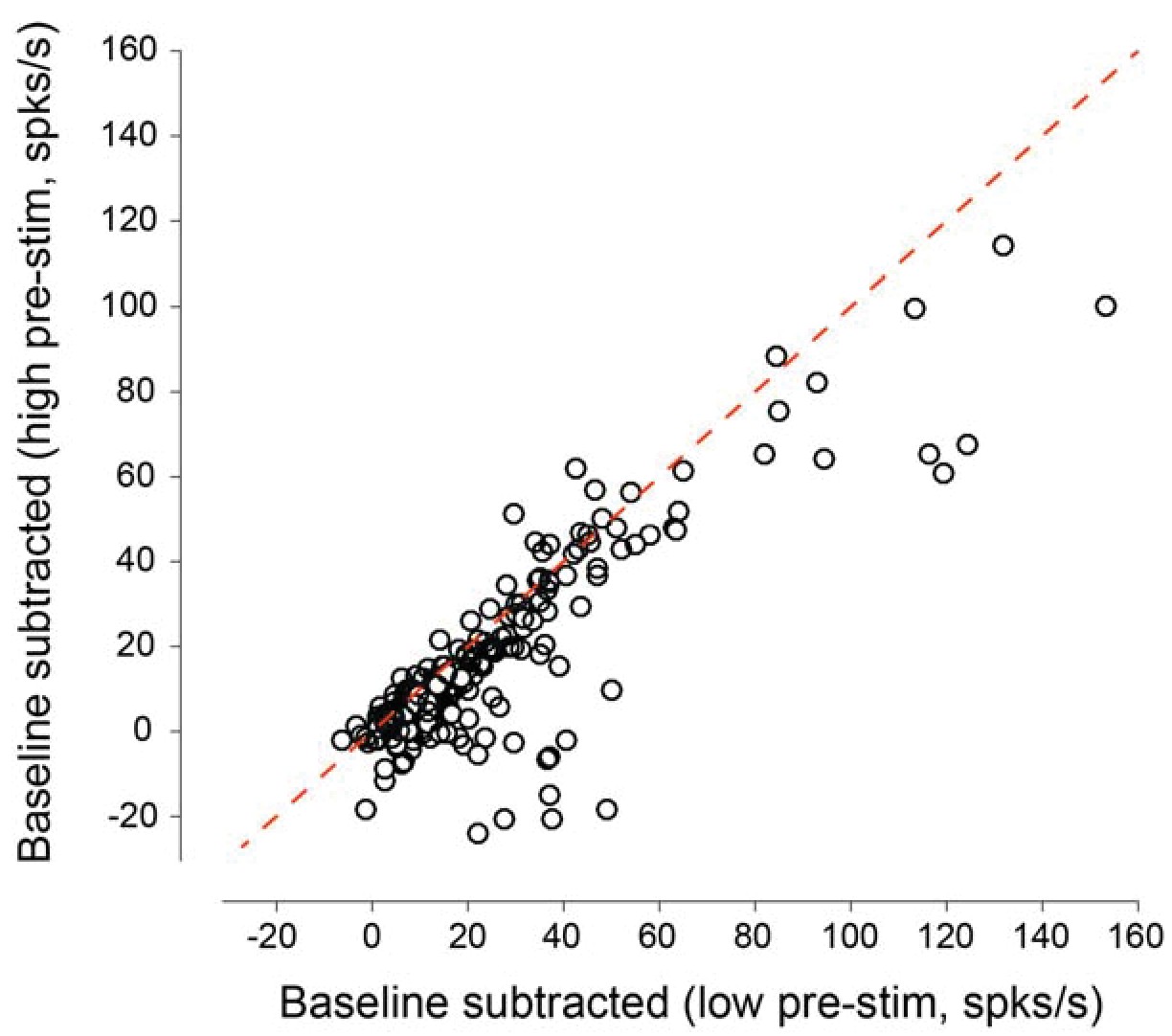
Baseline-subtracted evoked responses as a function of pre-stimulus response state for all the neurons recorded in the behavioral experiments.
Subtracting the 200 ms pre-stimulus activity from the evoked response reveals that the baseline-subtracted responses in the low pre-stimulus state are higher than those in the high pre-stimulus state (mean responses: 21.95 ± 1.58 vs. 14.88 ± 1.38 spks/s, p=4.73 10−16, paired t-test). The plot above indicates that evoked_low – baseline_low > evoked_high – baseline_high.This is equivalent to evoked_high – evoked_low < baseline_high – baseline_low. That is, fluctuations in evoked responses during wakefulness are smaller than the fluctuations in ongoing activity.
Figure 2
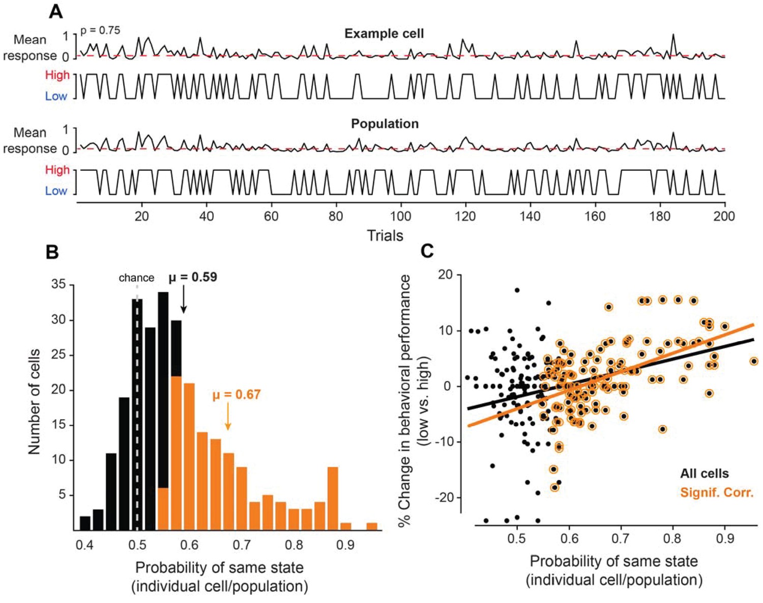
Neurons coupled with local population predict state-dependent changes in behavior.
(A) (Top) Firing rate of one example cell normalized between 0 and 1 for 200 trials. The red dotted line represents the median normalized firing rate. Trials with firing rates below the median are placed in the low pre-stimulus firing rate group and trials above the median are placed in the high pre-stimulus category. (Bottom) The mean firing rate of the remaining simultaneously recorded population of cells (excluding the example cell) for this example session, normalized between 0 and 1. Trials with firing rates below the median are placed in the low pre-stimulus firing rate group and trial above the median are placed in the high pre-stimulus group. For the example cell in panel A, the probability of sharing the same pre-stimulus state with the remaining population is p=0.75. (B) Histogram of the probability of same state (individual cells-population) for the entire set of cells for all sessions. The dotted line represents the chance probability level of 0.5 for a cell to share the same pre-stimulus state as the population. The mean probability is μ = 0.59, which is significantly greater than chance (p<0.0001, Wilcoxon rank-sum). The orange bars represent a sub-population of neurons that are significantly correlated to the population activity. The mean probability of the significantly correlated sub-population is μ = 0.67. (C) Percent change in behavioral performance (low vs. high pre-stimulus state) as a function of the probability of same pre-stimulus state for each neuron. Positive/negative numbers: behavioral performance is improved/impaired in the ‘low’ pre-stimulus state. The two variables are significantly correlated for all neurons (r = 0.36, p<10−8, Pearson correlation). The black line represents the linear regression fit (R2 = 0.13). The change in behavioral performance and probability of same pre-stimulus state were more correlated for the sub-population of neurons that are significantly correlated to the population response (r = 0.55, p<10−10, Pearson correlation). The orange line represents the linear regression fit (R2 = 0.30).
Figure 3 with 6 supplements
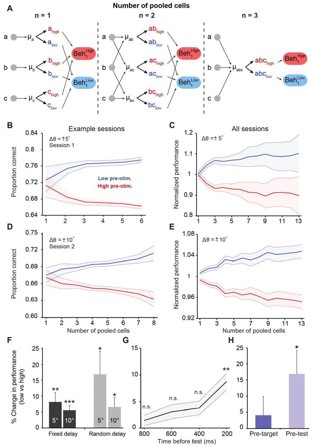
Cortical state influences behavioral performance in an orientation discrimination task.
(A) Diagram depicting our analysis linking neuronal populations and behavior (examples provided for n = 1, 2, and 3 cells). For n = 1, we computed the mean pre-stimulus firing rate individually for each neuron (μA, μB, and μC) and then calculated the average behavioral performance in the low and high pre-stimulus trials, averaged across the three cells for each group (Beh1low and Beh1high). For n = 2, we computed the mean normalized pre-stimulus activity for each pool of 2 cells (μAB, μAC, and μBC), then divided the trials into high and low groups, and calculated the average behavioral performance in the low and high pre-stimulus trials (Beh2low and Beh2high). For n = 3, we computed the mean normalized response for all three cells (μABC) and then split the trials to compare behavioral performance between the low and high pre-stimulus groups (Beh3low and Beh3high). (B–E) Behavioral performance is modulated by the ongoing population activity; a single session (panels B and D); all sessions (panels C and E). Behavioral performance associated with each ongoing activity state in each session was normalized by dividing the performance in each state by the average session performance (irrespective of pre-stimulus state). The pre-stimulus state was determined based on the pooled activity of neural populations of varying size (based on the method in panel A). The difference in discrimination performance between low and high pre-stimulus response states was greater when population size increases. Panels 3B and C correspond to orientation differences between target and test of ±5°; Panels 3D and E correspond to orientation differences between target and test of ±10°. ‘All sessions’ in panel C includes data from monkeys 1 and 2 (n = 24 sessions). ‘All sessions’ in panel E includes data from monkeys 1, 2, and 3 (n = 42 sessions). Error bars represent s.e.m of session performance for each population size. (F) Behavioral improvement in the low vs. high pre-stimulus conditions is present for both the fixed and random delay conditions for the ±5° and ±10° orientation differences (*p<0.05, **p<0.01, ***p<0.001; Wilcoxon signed-rank test). Results in panels F-H were obtained for a population size of 5 to include most sessions in the analysis. (G) Behavioral improvement in the low vs. high pre-stimulus state for different pre-stimulus periods. The x-axis represents the time relative to the onset of the test stimulus. Pre-stimulus state was assessed based on the pre-stimulus interval in 200 ms steps (during the delay period). The improvement in discrimination performance in the low pre-stimulus state occurs only during the 200 ms period before test presentation. (**p<0.01; n.s. = non significant; Wilcoxon signed-rank test). Error bars represent s.e.m. (H) Neuronal activity in the pre-test interval influences behavior to a larger extent than that in the pre-target interval (*p<0.05; n = 13 sessions from the random delay experiment; the fixed delay data was not included because the pre-target interval was too small, that is, 100 ms).
Figure 3—figure supplement 1
Cortical state influences behavioral performance in an orientation discrimination task (fixed delay experiments).
Three monkeys were trained in a behavioral task as shown in Figure 1A. Behavioral performance was modulated by the pre-stimulus (test) response state; single sessions (panels A–B); all sessions (panels C–D). Upper panels in (A) and (C) correspond to orientation differences between target and test of ± 5°; lower panels correspond to orientation differences between target and test of ± 10°. Behavioral performance was higher in the low pre-stimulus activity group (p<0.0001), Wilcoxon rank-sum at highest population level; F(1,103)=23.3; p<0.0001; two-way repeated measures ANOVA) for ±5° orientation discrimination. Similar results were found for the ±10° discrimination experiment (p<0.0001, Wilcoxon rank-sum at highest population level; F(1,425)=104.4; p<0.0001, two-way repeated measures ANOVA). Panel (C) includes data from monkeys 1 and 2; panel (D) includes data from monkeys 1, 2, and 3. Error bars represent s.e.m of session performance for each neural population size.
Figure 3—figure supplement 2
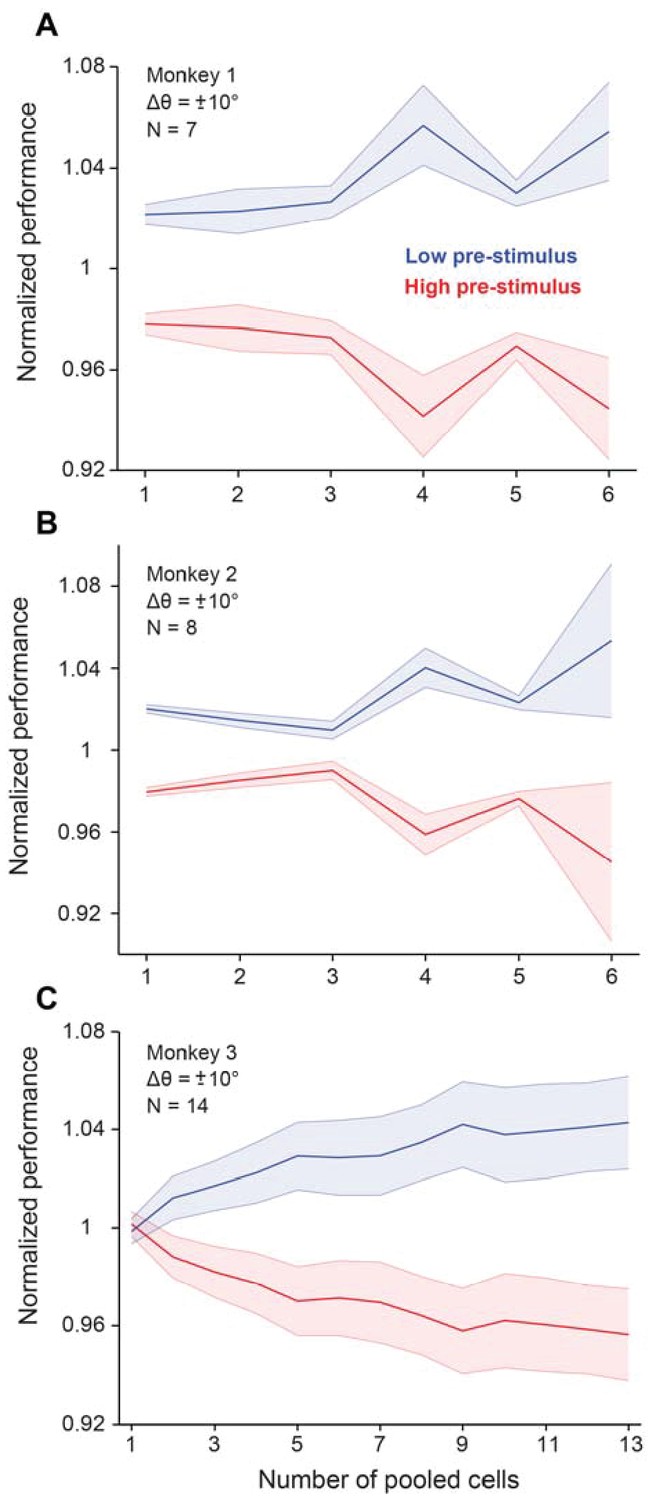
Cortical state influences behavioral performance in an orientation discrimination task (results shown for each monkey trained in the fixed delay experiments).
When the neural population is in the low pre-stimulus state, each monkey performs significantly better compared to when the neural population is in the high pre-stimulus state (p<0.005, Wilcoxon rank-sum at highest population level, F(Azouz and Gray, 2003; Cohen and Maunsell, 2009a)=63.7; p<0.0001, two-way repeated measures ANOVA; p<0.0001, Wilcoxon rank-sum at highest population level, F(Azouz and Gray, 2003; Crochet et al., 2005)=75.8; p<0.001, two-way repeated measures ANOVA; p<0.005, Wilcoxon rank-sum at highest population level, F(1,279)=47.9; p<0.0001; two-way repeated measures ANOVA, respectively). These results represent behavioral performance in the fixed delay experiments. Error bars represent s.e.m.
Figure 3—figure supplement 3
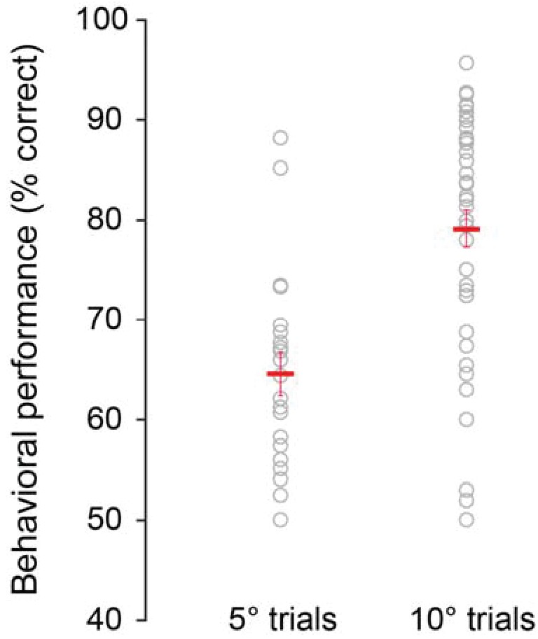
Behavioral performance depends on task difficulty.
Animals performed more poorly when they discriminated small orientation differences (±5o; mean across sessions: 64.58 ± 2.19% correct responses) compared to larger orientation differences (±10o; mean across sessions: 79.17 ± 1.85% correct responses, p=4.03 10−5, rank-sum test). Each circle represents one session. Red crosses mark the mean performances across sessions.
Figure 3—figure supplement 4
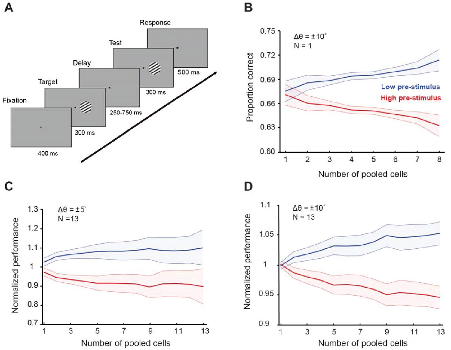
Cortical state influences behavioral performance in an orientation discrimination task (results shown for the random delay experiments).
(A) One monkey was trained in an orientation discrimination task with a random delay between target and test presentation (in the 250–750 ms range). Behavioral performance was modulated by the pre-stimulus response state before test presentation. Example of a single session (B) and normalized behavioral performance for all recorded sessions for ± 5° (C) and ±10° (D) discriminations. The responses of each neuron were grouped depending on the level of pre-stimulus activity into ‘low’ and ‘high’ groups. Behavioral performance was higher in the low pre-stimulus response group for the ±5° discrimination trials (p<0.05, Wilcoxon rank-sum at highest population level; F(1,259)=42.14, p<0.0001; two-way repeated measures ANOVA). Similar results were found when the target-test orientation difference was ±10° (p<0.005, Wilcoxon rank-sum at highest population level; F(1,251)=55.7; p<0.0001, two-way repeated measures ANOVA). The total number of neurons used for this analysis was 103; the figure represents data from Monkey four in our study. Error bars represent the s.e.m. of session performance for each population size.
Figure 3—figure supplement 5
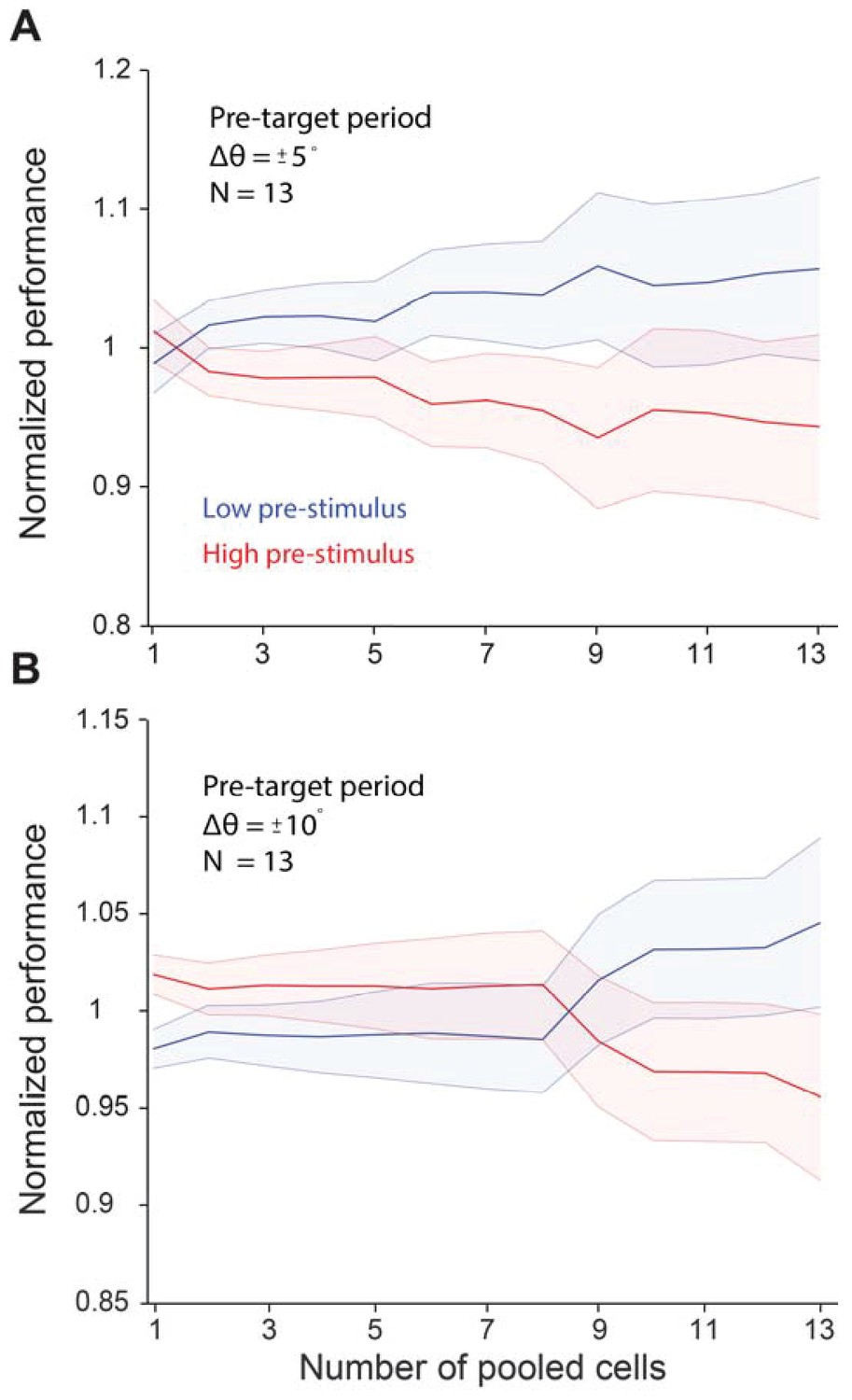
Pre-target neural activity does not influence behavioral performance in a significant manner.
Behavioral performance was higher in the low pre-target response state when the relative difference between the target and test (Δθ) was ± 5° (p=0.40, Wilcoxon rank-sum at highest population level). We did not find a significant difference when Δθ was ± 10° (p=0.09, Wilcoxon rank-sum at highest population level). The five degree orientation data includes data from monkeys 1 and 2. The 10 deg data includes data from monkeys 1, 2, and 4. Error bars represent s.e.m.
Figure 3—figure supplement 6
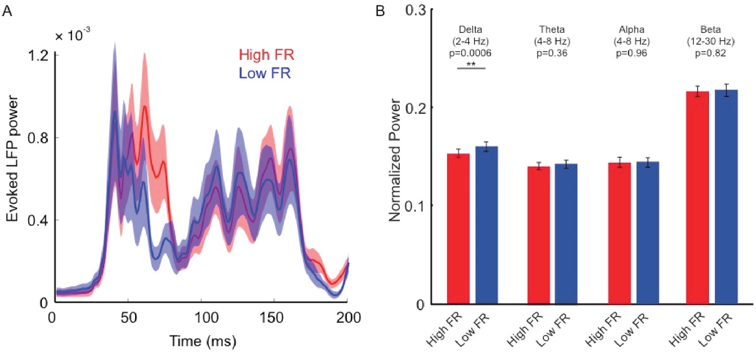
Relationship between LFP power and pre-stimulus response state.
(A) Relationship between pre-stimulus response state (low vs. high pre-stimulus firing rate, FR) and evoked LFPs. Trials were sorted into high and low pre-stimulus firing groups based on neural activity 0–200 ms before stimulus presentation. The two response traces represent the mean LFP total power across electrode contacts and sessions for the low and high pre-stimulus states (low and high FR). We did not find statistically significant differences in evoked LFPs during test stimulus presentation (p=0.21, 2-way repeated measures ANOVA). (B) We further sorted the LFP signal into different physiological frequency bands and calculated the LFP power in each band. We examined whether the LFP power in specific physiological frequency bands is influenced by pre-stimulus activity. Across our recording contacts and sessions, we only found a small, significant, difference in the upper portion of delta band (2–4 Hz, p=0.0006, Wilcoxon rank-sum). However, there were no statistically significant effects between the two groups for alpha (8–12 Hz), theta (4–8 Hz), and beta (12–30 Hz) frequency bands (p>0.05, Wilcoxon rank-sum). Each bar represents the mean normalized LFP power for each cortical state and frequency condition. Error bars represent s.e.m.
Figure 4
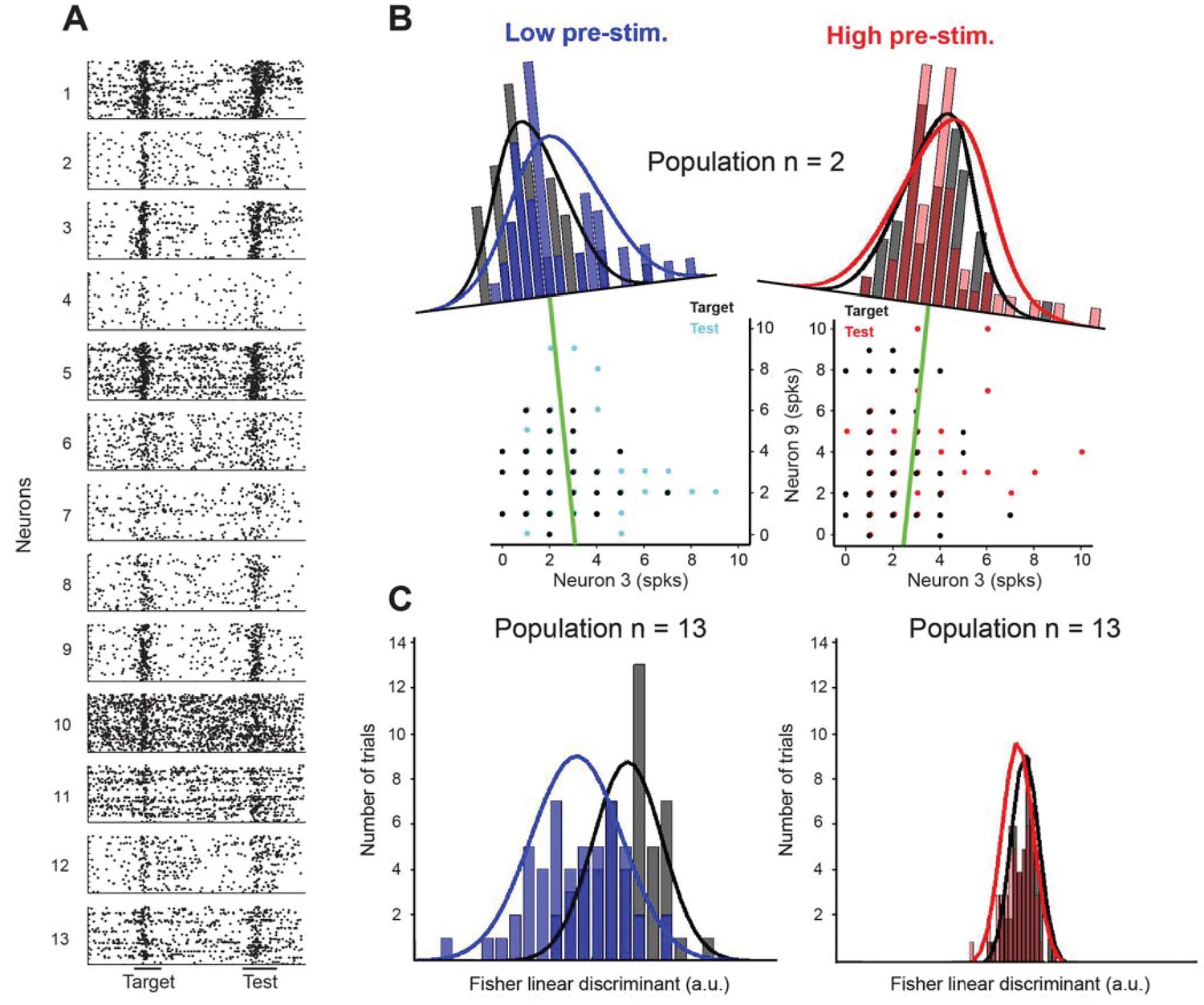
Fisher linear discriminant (FLD) analysis for one example session.
(A) Raster plots for 13 cells recorded simultaneously in a session. Each dot represents the time of an action potential. Horizontal bars at the bottom represent stimulus duration for target and test. The random delay period has been truncated to align the test responses. (B) Example FLD of one cell pair (neurons 3 and 9). Each circle represents the total number of spikes elicited during the target or test stimulus. Each histogram is plotted on the Fisher linear discriminant axis which maximizes the difference between target and test relative to the variance of the responses. The black and blue (black and red for the high pre-stimulus condition) curves represent one-dimensional Gaussian fits for the target and test distributions, respectively. The green line represents the decision boundary. (C) Example FLD for the full population of 13 cells. There is a greater difference between the two distributions in the low pre-stimulus trials compared to the high pre-stimulus trials.
Figure 5 with 1 supplement
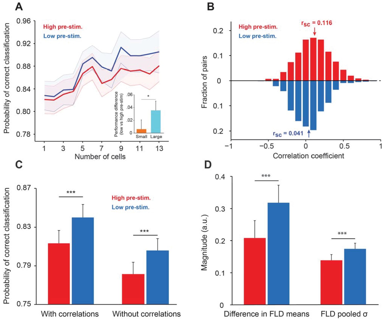
Cortical state influences the information encoded in population activity.
(A) The probability of correct classification (PCC) as a function of population size. PCC was significantly higher in the low pre-stimulus case (F(1,164)=9.32; p<0.005; two-way repeated measures ANOVA). (inset) The difference in classification performance between low and high pre-stimulus response states for a small (n = 2, orange) and a large population (n = 12, blue). The performance difference was greater for the larger neural population (p<0.05, bootstrap test). (B) Noise correlations of evoked responses for the high and low pre-stimulus states – correlations were significantly higher in the high pre-stimulus state (p=7.918e-10; paired t-test). (C) Probability of correct classification for the two cortical states. ‘With correlations’ represents data using the following equation: ; Probability of correct classification = . ‘Without correlations’ represents the probability of correct classification when ignoring the effect of noise correlations using (), where is the diagonal covariance matrix. In each condition there is a statistically significant difference between the high and low pre-stimulus conditions (*p<0.05; paired t-test). (D) The magnitude of the difference in FLD means (left) and the magnitude of the pooled standard deviation () of the FLD (right). In the low pre-stimulus condition, the difference in means was significantly greater (p<0.0001; paired t-test). The average variance was also higher in the low pre-stimulus condition (p<0.0001; paired t-test), but this had less overall impact on the population d’. The results in this figure were obtained for all the cells recorded across sessions for an orientation difference of ±5°.
Figure 5—figure supplement 1
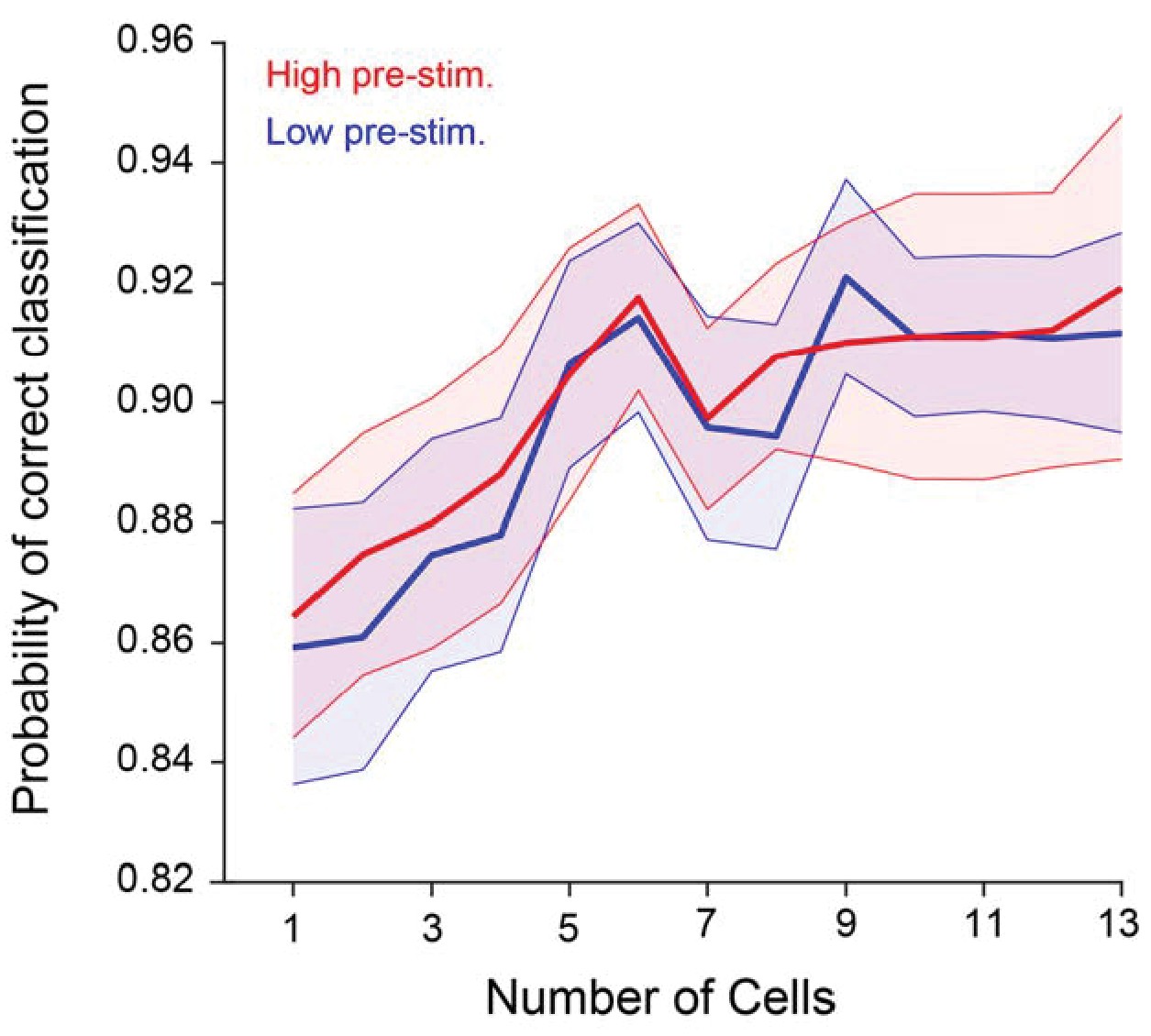
Probability of correct classification (PCC) as a function of population size when baseline-subtracted evoked responses to the target and test stimuli are used.
PCC does not depend significantly on pre-stimulus activity for any population size (p>0.1; two-way repeated measures ANOVA).
Additional files
-
Transparent reporting form
- https://doi.org/10.7554/eLife.29226.018
Download links
A two-part list of links to download the article, or parts of the article, in various formats.
Downloads (link to download the article as PDF)
Open citations (links to open the citations from this article in various online reference manager services)
Cite this article (links to download the citations from this article in formats compatible with various reference manager tools)
Cortical response states for enhanced sensory discrimination
eLife 6:e29226.
https://doi.org/10.7554/eLife.29226


