Removal of inhibition uncovers latent movement potential during preparation
- University of Pittsburgh, United States
Figures
Figure 1
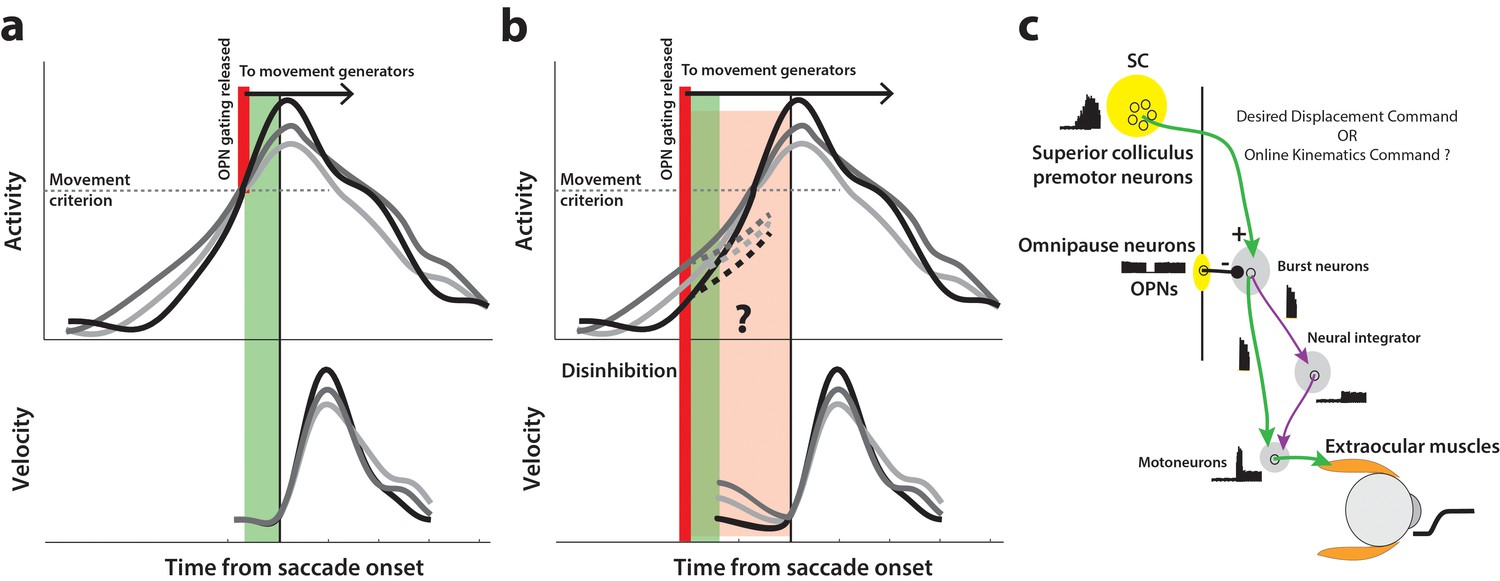
Conceptual schematic of saccade and pre-saccade motor potential revealed by disinhibition.
(a) Under normal conditions, premotor activity accumulates at different rates on different trials (three example traces in top row) to a movement initiation criterion, opening downstream gating (thick red line) and triggering the saccade following an efferent delay (~20 ms, green window). Following saccade onset, variation in neural activity is correlated with variation in saccade velocity (match gray scale in top and bottom rows), indicating the neuron’s motor potential. (b) Removal of inhibition through an experimental manipulation at an earlier time (thick red line), during saccade preparation and before the typical movement criterion is reached. The disinhibition may reveal the motor potential of ongoing activity in the form of correlated kinematics of the eye before onset of the actual saccade (light red region, velocity traces in bottom row), and also allows us to study any changes in the dynamics of activity leading up to the reduced latency saccades (dashed activity traces in top row). (c) Schematic of the premotor circuitry involved in saccade generation. A desired displacement command (or, as tested here, a kinematics-driving command) is sent from neurons in SC to the burst neurons in the brainstem reticular formation (also referred to as the burst generator). This pathway is gated by tonic inhibition from the OPNs under normal conditions. Approximately 20 ms before saccade onset, OPN activity pauses, disinhibiting the burst neurons and allowing the excitatory pathway (green arrows) to actuate an eye movement. This study tests whether disinhibiting the pathway downstream of SC by blink-induced suppression of OPNs results in an immediate eye movement.
Figure 2
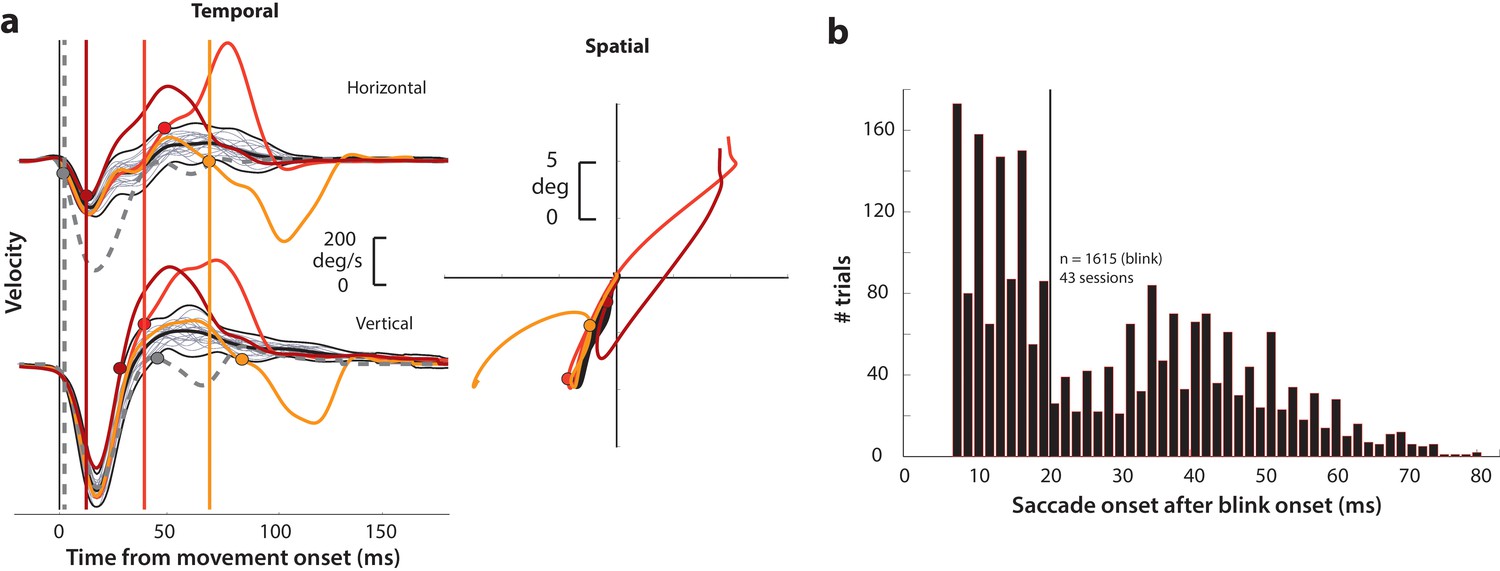
Determining goal-directed saccade onset in blink-triggered eye movements.
(a) Left column: horizontal (top row) and vertical (bottom row) eye velocity profiles during blink-related eye movements obtained during fixation (BREMs, thin gray traces) and three example blink-triggered saccadic eye movements (colored traces) from one session. The thick black trace in the middle of the BREM profiles is their mean and the two black traces above and below it are 2.5 s.d. bounds. Saccade onset was determined to be the point where an individual velocity profile (colored traces) crossed the BREM bounds and stayed outside for 15 consecutive time points. This point was determined independently for the horizontal and vertical channels (colored circles corresponding to each trace in the two rows), and the earlier time point was taken as the onset of the overall movement (vertical colored lines). The dashed gray velocity profile that deviates from the BREM very close to movement onset (<5 ms) is shown to highlight a case where the saccade starts before being perturbed by the blink, and was not considered as a blink-triggered movement in this study. Right column: Spatial trajectories of the eye for the three example blink-triggered movements from the left column, with the corresponding saccade onset time points indicated by the circles. The trajectory of the BREM template is shown in black (for the sake of clarity, only the mean is shown). Note that the movements in this session were made to one of two possible targets on any given trial. (b) Distribution of goal-directed saccade onset times relative to overall movement onset for blink-triggered movements (n = 1615) across all sessions (n = 43). For the motor potential and accumulation rate analyses (Figures 4–5 and 7), we only considered movements where the blink-triggered saccade started at least 20 ms after overall movement onset (to the right of the vertical line). For the threshold analysis (Figure 6), we considered all blink-triggered movements.
Figure 3
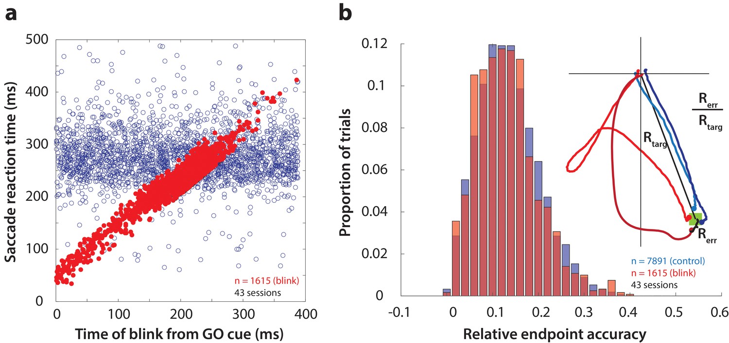
Time course and accuracy of blink-triggered saccades.
(a) Saccade reaction time as a function of blink onset time across all trials (n = 7891 control trials, 1615 blink trials) and sessions (n = 43). Red filled circles are individual blink trials, and blue circles are from control trials with randomly assigned blink times for comparison. For visualization alone, only a random selection of control trials equal in number to blink trials are plotted. (b) Endpoint accuracy for control and blink-triggered movements (blue and red histograms, respectively) across all trials from all sessions. To enable comparison across movement amplitudes, the endpoint error was normalized as the actual Euclidean endpoint error from the target divided by the eccentricity of the target, as depicted in the spatial plot in the inset.
Figure 4 with 1 supplement
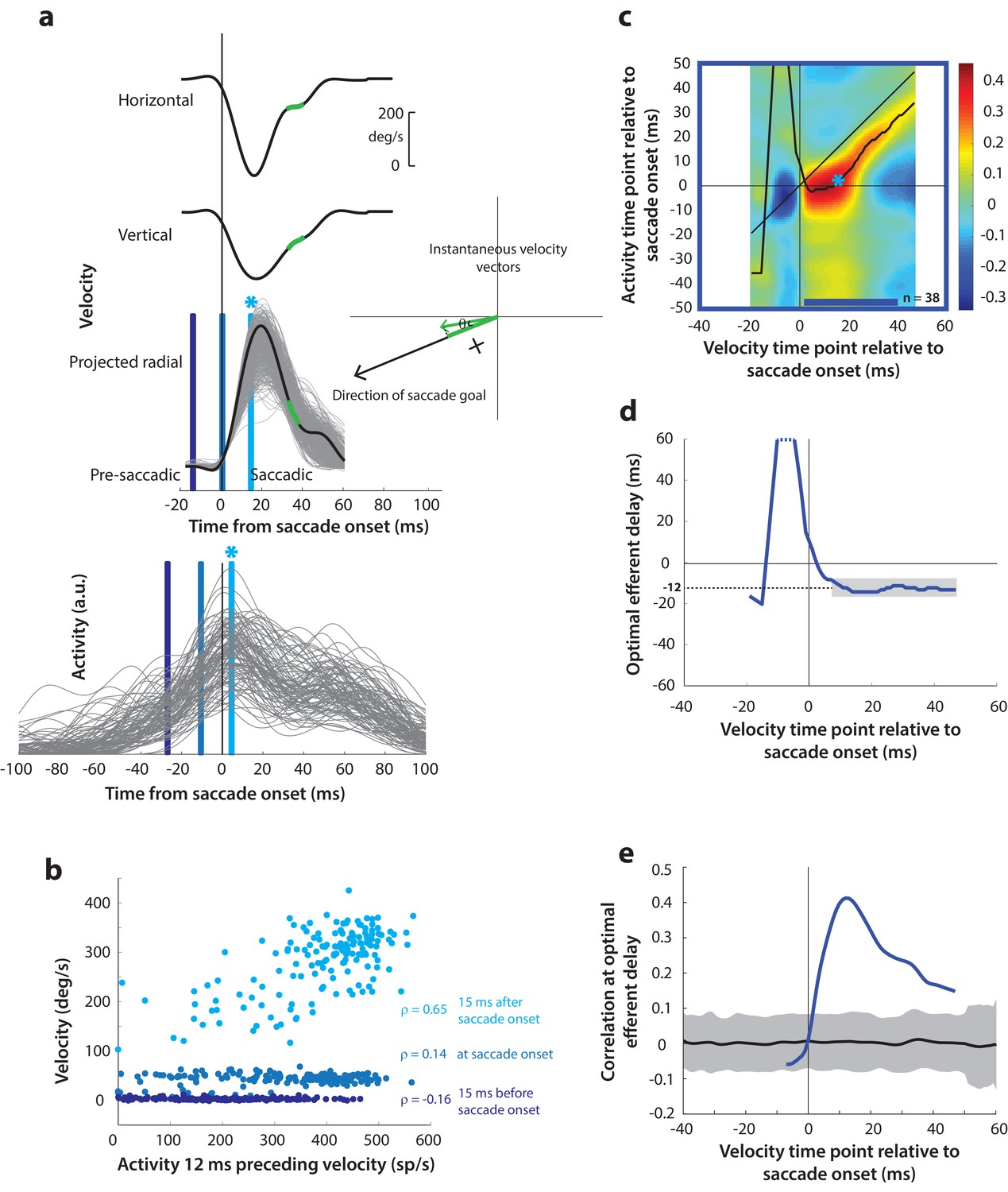
Motor potential during control saccades.
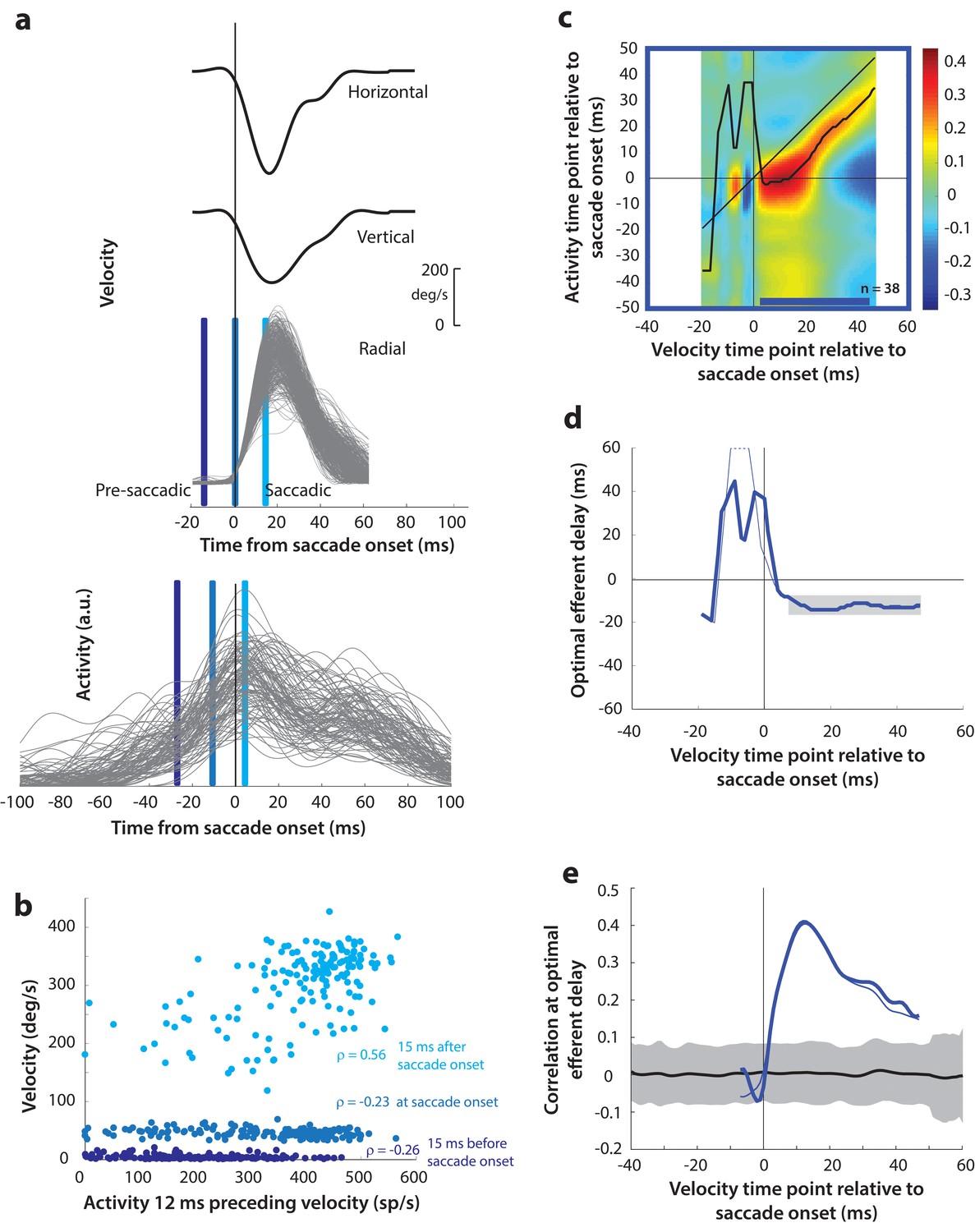
(a) Estimating motor potential as correlation between neural activity and saccade kinematics. Horizontal and vertical velocity traces (top two rows) on control trials are converted to radial velocity (third row) in the direction of the saccade goal. The projection of the green vector in the inset and the corresponding green parts of the velocity traces illustrate this computation. One trial (thick black trace) is highlighted for clarity. For control trials, the projected and executed vectors are very similar. The bottom row shows neural activity traces on different trials for the neuron recorded in this example session. (b) Motor potential is estimated as the correlation between neural activity and projected saccade kinematics. The scatter plot of the projected radial velocity 15 ms after saccade onset, at saccade onset, and 15 ms before saccade onset (light, medium, and dark blue points, respectively, and corresponding vertical lines in panel a) against neural activity 12 ms preceding the velocity time points shows that the neuron has motor potential once the saccade has started (Pearson’s correlation coefficient = 0.65). Each point corresponds to one trial. (c) Point-by-point correlation between velocity and activity, averaged across neurons. Heat map colors represent correlation values. As an example, the light blue asterisk refers to the correlation between the velocity and activity corresponding to the time points with the asterisk in panel a. The black curve traces the contour of the highest correlation time points in the activity for each point during the movement. The blue bar at the bottom of the heatmap indicates timepoints at which the average correlation was significant (based on 95% CI from panel e). (d) Optimal efferent delay computed as the distance of the black trace in panel c from the unity line. Negative values for the delay are causal, i.e., correlation was high for activity points leading the velocity points. The shaded gray bar shows that the optimal delay was consistent during the movement (mean for shaded region = −12 ms) (e) Population average correlation as a function of time at the −12 ms estimated efferent delay. The black trace is the mean and the gray region is the 95% confidence interval for the bootstrapped (trial-shuffled) correlation distribution.
Figure 4—figure supplement 1
Motor potential during control saccades, computed with raw velocities.
(a) As in Figure 4a, horizontal and vertical velocity traces (top two rows) on control trials are converted to radial velocity (third row). In contrast to Figure 4a, the velocities are used as is to compute motor potential, without projecting onto the direction of the saccade goal. The bottom row shows neural activity traces on different trials for the neuron recorded in this example session (same as Figure 4a). (b) Motor potential is estimated as the correlation between neural activity and saccade kinematics in appropriate time windows. The scatter plot of the projected radial velocity 15 ms after saccade onset, at saccade onset, and 15 ms before saccade onset (light, medium, and dark blue points, respectively, and corresponding vertical lines in panel a) against neural activity 12 ms preceding the velocity time points. Each point corresponds to one trial. (c) Point-by-point correlation of velocity and activity, averaged across neurons. The black curve traces the contour of the highest correlation time points in the activity for each point during the movement. The blue bar at the bottom of the heatmap indicates timepoints at which the average correlation was significant (based on 95% CI from panel e). (d) Optimal efferent delay (thick blue trace) computed as the distance of the black trace in panel c from the unity line. Negative values for the delay are causal, that is, correlation was high for activity points leading the velocity points. The gray bar shows that the optimal delay was consistent during the movement (−12 ms) (e) Population average correlation as a function of time at the −12 ms estimated efferent delay. The black trace is the mean and the gray region is the 95% confidence interval for the bootstrapped (trial-shuffled) correlation distribution. The thin traces in panels d-e are from Figure 4d–e, overlaid for comparison.
Figure 5 with 2 supplements
Motor potential on blink trials.
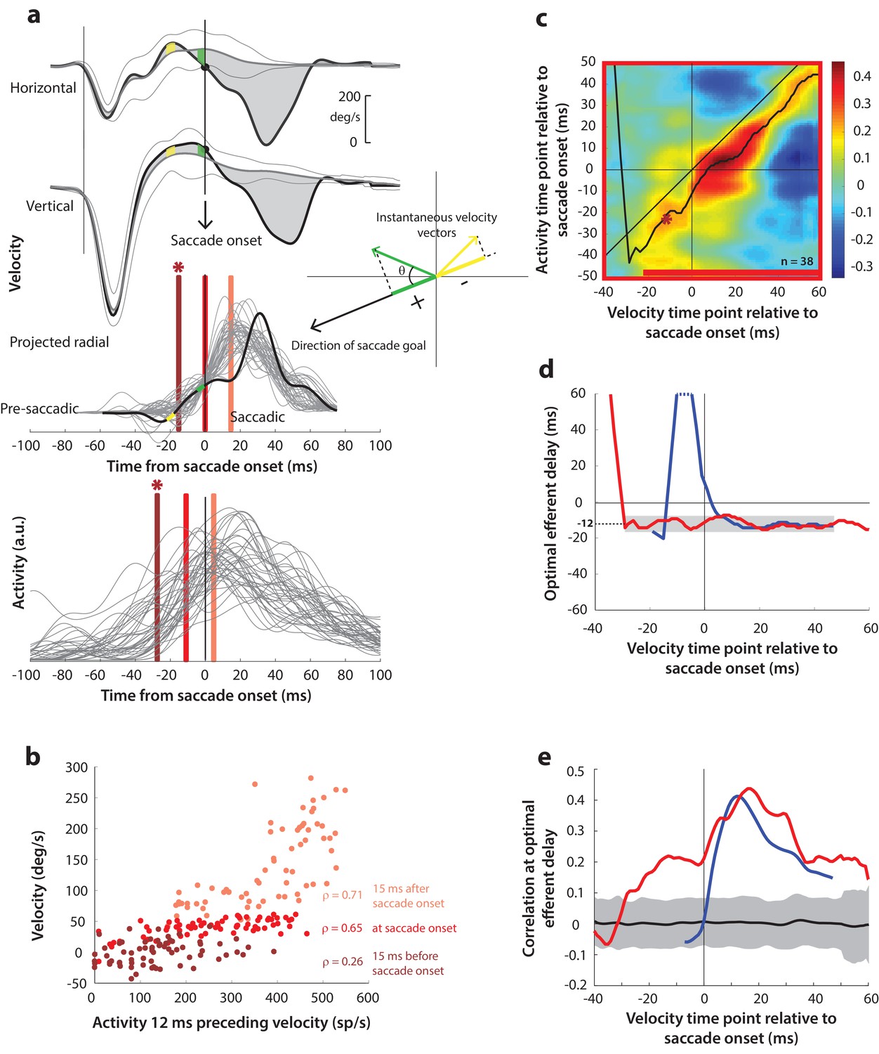
(a) Computation of the kinematic variable for blink-triggered movements. Horizontal and vertical velocities (thick black traces in top two rows) are converted to residual velocities (gray fill) after subtracting the corresponding mean BREM template (middle thin black trace in top two rows), in order to discount the effects of intrinsic variability in the BREM itself. The radial residual velocity (third row) in the direction of the saccade goal is then computed, similar to Figure 4a. The green and yellow time points in the velocity traces (shown as thicker than an instant for clarity), represented as corresponding velocity vectors in the inset, illustrate this process. For example, the green velocity residual, immediately before saccade onset, deviates negatively from the BREM in the horizontal component, and positively in the vertical component, resulting in an instantaneous kinematic vector pointing leftwards and upwards. The component of this vector in the direction of the saccade goal is then taken as the kinematic variable for this time point (also compare Figure 5—figure supplement 1). (b) Scatter plot of the neural activity versus velocity at the three indicated time points (red points of various saturation, at corresponding red lines in panel a) for blink-triggered movements. As in Figure 4b, these are plotted at the −12 ms shift between activity and velocity Note the strong correlation for pre-saccade time points compared to Figure 4b. (c) Point-by-point correlation of projected residual velocity with activity, averaged across neurons, for blink-triggered movements. The velocity time points are with respect to time of saccade onset extracted from the blink-triggered movement. The dark red asterisk points to the correlation between the velocity and activity corresponding to the time points with the asterisk in panel a. The black curve traces the contour of the highest correlation time points in the activity for each point during the movement. The red bar at the bottom of the heatmap indicates timepoints at which the average correlation was significant (based on 95% CI from panel e). (d) Optimal efferent delay computed as the distance of the black trace in panel c from the unity line. The red trace is for blink-triggered movements, and the blue trace is from Figure 4d for control saccades, overlaid for comparison. Negative values for the delay are causal, i.e., correlation was high for activity points leading the velocity points. The gray bar highlights the fact that the optimal delay was consistent during both control and blink-triggered saccades, and both before and after saccade onset for the latter (mean for shaded region = −12 ms). (e) Population average correlation for blink-triggered movements (red trace) as a function of time at the −12 ms estimated efferent delay. The blue trace is from Figure 4e for control saccades, overlaid for comparison. The black trace is the mean and the gray region is the 95% confidence interval for the bootstrapped (trial-shuffled) correlation distribution.
Figure 5—figure supplement 1
Motor potential on blink trials, computed with raw velocities.
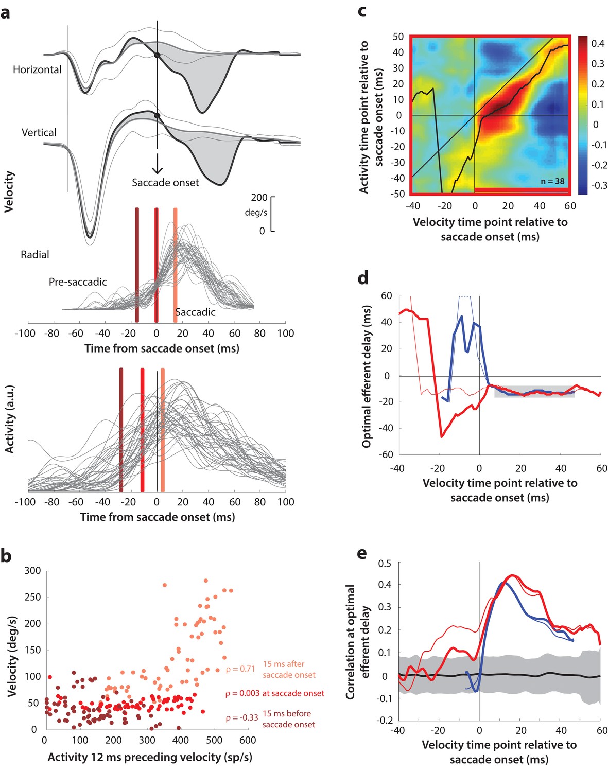
(a) As in Figure 5a, horizontal and vertical velocity traces (top two rows) during blink-triggered movements are converted to radial velocity (third row). In contrast to Figure 5a, the residual velocities (gray shaded deviation from the BREM template) are used as is to compute motor potential, without projecting onto the direction of the saccade goal. The bottom row shows neural activity traces on different trials for the neuron recorded in this example session (same as Figure 5a). (b) Scatter plot of the neural activity versus velocity at the three time points (shaded red windows) from panel a for blink-triggered movements. (c) Point-by-point correlation of velocity and activity, averaged across neurons, for blink-triggered movements. The velocity time points are with respect to time of saccade onset extracted from the blink-triggered movement. The black curve traces the contour of the highest correlation time points in the activity for each point during the movement. The red bar at the bottom of the heatmap indicates timepoints at which the average correlation was significant (based on 95% CI from panel e). (d) Optimal efferent delay computed as the distance of the black trace in panel c from the unity line. The thick red trace is for blink-triggered movements computing using raw kinematics, and the others are from previous analyses overlaid for comparison (thin red trace is from Figure 5d, thick blue trace is from Figure 4—figure supplement 1d, and thin blue trace is from Figure 4d). Negative values for the delay are causal, i.e., correlation was high for activity points leading the velocity points. The estimated efferent delay after saccade onset was consistent with the result in Figure 5 (mean for shaded region = −12 ms), but note the abrupt deviation from this value in the pre-saccade period, compared to the thin red trace. (e) Population average correlation for blink-triggered movements (thick red trace) as a function of time at the −12 ms estimated efferent delay. As in panel d, the other traces are from previous analyses, overlaid for comparison. The black trace is the mean and the gray region is the 95% confidence interval for the bootstrapped (trial-shuffled) correlation distribution.
Figure 5—figure supplement 2

‘Main sequence’ velocity-amplitude relationship.
(a) Peak velocity of the saccadic component of blink-triggered movement as a function of movement amplitude. Each point represents one trial. Points are colored by individual subjects, but since the range of amplitudes was much smaller for one subject (red points), the regression was computed on all points taken together. (b) Mean projected residual velocity in a 20 ms window before saccade onset as a function of movement amplitude. Note the weaker but still significant positive relationship between velocity and amplitude.
Figure 6
Analysis of putative threshold.
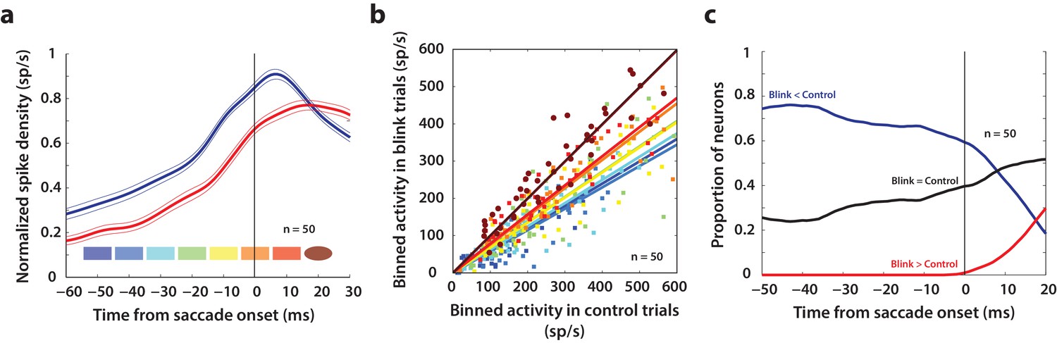
(a) Average normalized population activity (thick traces) aligned on saccade onset for control (blue trace) and blink (red trace) trials. The thin lines represent s.e.m. The colored swatches at the bottom show the time windows used for the analysis presented in b; their shapes represent the presence (rectangle) or absence (ellipse) of a significant difference between control and blink rates in that time window. (b) Scatter plot of the activities of individual neurons (n = 50) in the time windows illustrated in (a) for control versus blink trials (each set of colored points corresponds to one time window). Square points indicate that the activity in control trials was higher in that window compared to blink trials, and circles indicate that there was no significant difference between the two conditions. Colored lines indicate linear fits to the scatter at the corresponding time window. The diagonal (thin black line) is the unity line; it overlaps with the dark brown line. (c) Proportion of neurons exhibiting the corresponding labelled differences between the two conditions as a function of time.
Figure 7
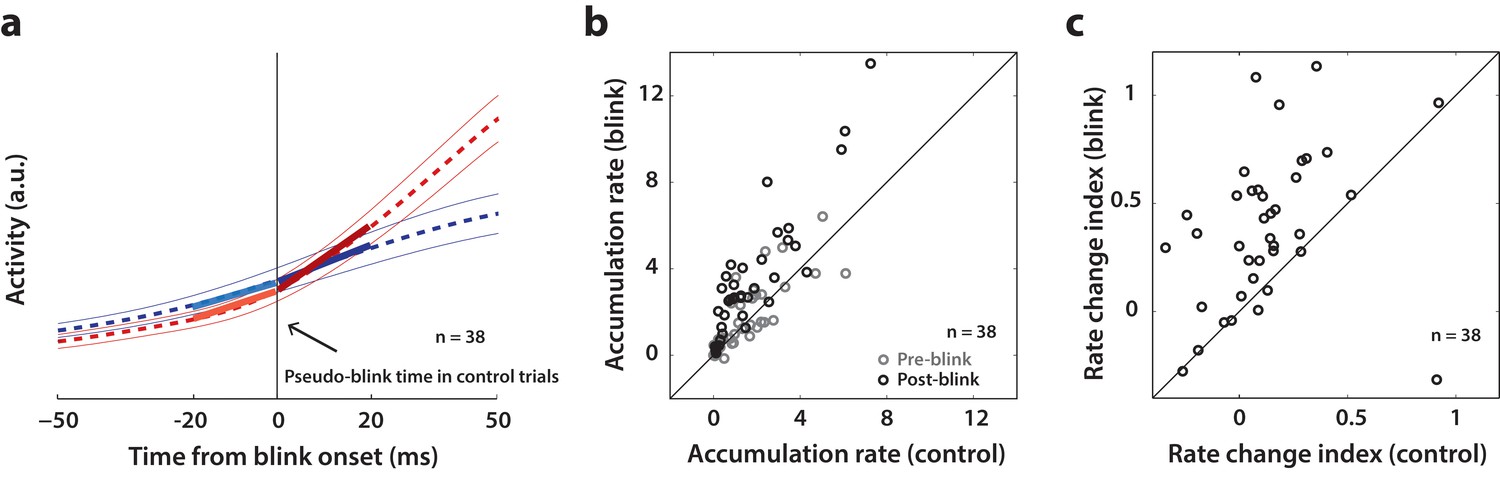
Analysis of accumulation rate change following perturbation.
(a) Schematic illustrating the computation of accumulation rates before and after the blink. The snippet shows the average population activity (dashed lines) s.e.m (thin lines) centered on blink onset for blink trials (red trace) and pseudo-blink onset from the surrogate dataset for control trials (blue trace). The thick lines represent linear fits to the activity 20 ms before (lighter colors) and after (dark colors) the blink time. (b) Scatter plot of pre-blink (gray circles) and post-blink (black circles) accumulation rates (slopes of fits shown in panel a) of individual neurons for control versus blink trials. The unity line is on the diagonal. (c) Scatter plot of the pre-to-post rate modulation index for control versus blink trials.
Author response image 1
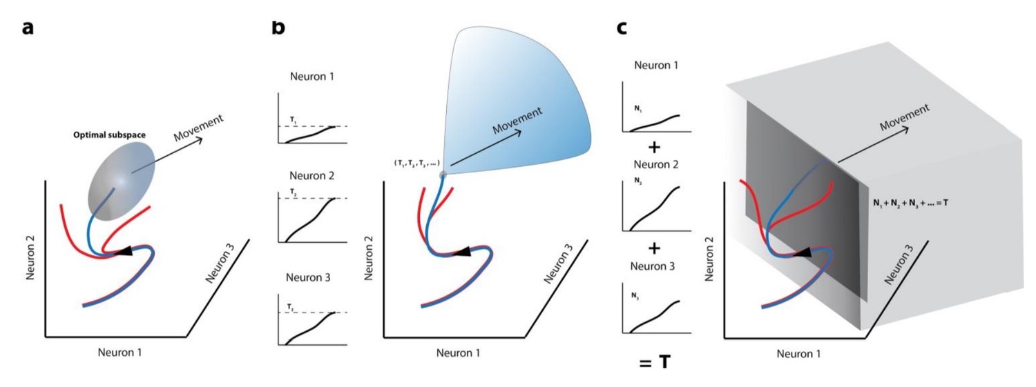
Movement initiation models in the population dynamics framework.
In all cases, population activity is represented as an evolving trajectory in multi-dimensional space – only the activity of 3 neurons/3 latent dimensions are displayed. (a) The optimal/potent subspace hypothesis suggests that movements are triggered when population activity reaches a pre-determined activity subspace (ellipsoid). Thus, only the blue trajectory will result in movement generation whereas trajectories that don’t reach this “optimal” subspace (red trajectories) don’t lead to movements. (b) The classic version of the threshold hypothesis posits that movements are initiated when the activity of individual neurons reaches a threshold level (3 different levels shown in left column). When represented collectively in a population framework, this is equivalent to a point in multidimensional space, which must be crossed to generate a movement, making it a far narrower “optimal subspace” equivalent. (c) Recent iterations of the threshold hypothesis expand the classic version to allow for a threshold at the population level, represented by a linear combination of individual neuron activities. This is equivalent to crossing a hyperplane in multi-dimensional space. Note that in all these cases, activity must cross some decision boundary (subspace bounds, point, or plane) in order to generate a movement (blue trajectories), implying that the set of activities prior to this point lacks the potential to do so.
Author response image 2
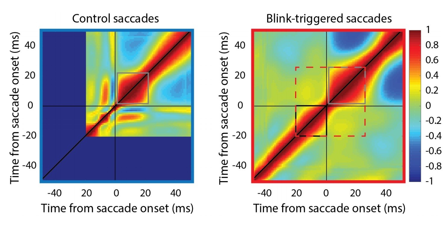
Self-correlation of velocity profiles.
Left – Across-trial correlated variability of instantaneous velocity on control trials. These correlations are computed similarly to the activity-velocity correlations in Figures 4C and 5C, except with the activity replaced by velocity. Smooth and continuous velocity profiles result in a window of high correlations (gray square) where the velocity values are correlated amongst themselves. Right – For blink trials, the velocity profiles are correlated with each other over time after saccade onset (gray square), and separately, before saccade onset (black square, during the epoch of preparatory motor potential), with a discontinuity in between (narrowing of correlations along the diagonal). It is important to note that the correlation between pre-saccade and post-saccade velocities is not nearly as strong (if they were, one would expect a window of high correlations marked by the dashed red square). Moreover, if saccade onset were over- or under- estimated, either the black or gray windows should’ve crossed the zero point.
Additional files
-
Transparent reporting form
- https://doi.org/10.7554/eLife.29648.013
Download links
A two-part list of links to download the article, or parts of the article, in various formats.
Downloads (link to download the article as PDF)
Open citations (links to open the citations from this article in various online reference manager services)
Cite this article (links to download the citations from this article in formats compatible with various reference manager tools)
Removal of inhibition uncovers latent movement potential during preparation
eLife 6:e29648.
https://doi.org/10.7554/eLife.29648


