A new genus of horse from Pleistocene North America
- University of California, Santa Cruz, United States
- Tromsø University Museum, UiT - The Arctic University of Norway, Norway
- Government of Yukon, Canada
- American Museum of Natural History, United States
- Cogstone Resource Management, Incorporated, United States
- California State University San Bernardino, United States
- Harvard University, United States
- German Consortium for Translational Cancer Research, Germany
- University of Alaska Fairbanks, United States
- Natural History Museum of Denmark, Denmark
- Université Paul Sabatier, Université de Toulouse, France
- University of California, Irvine, United States
- University of Alberta, Canada
Figures
Figure 1 with 3 supplements
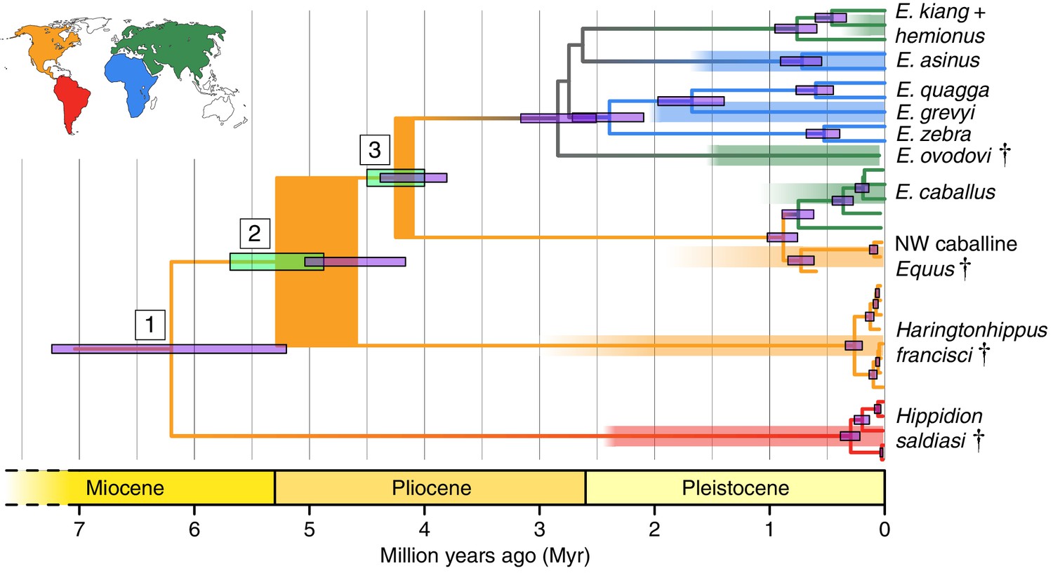
Phylogeny of extant and middle-late Pleistocene equids, as inferred from the Bayesian analysis of full mitochondrial genomes.
Purple node-bars illustrate the 95% highest posterior density of node heights and are shown for nodes with >0.99 posterior probability support. The range of divergence estimates derived from our nuclear genomic analyses is shown by the thicker, lime green node-bars ([Orlando et al., 2013]; this study). Nodes highlighted in the main text are labeled with boxed numbers. All analyses were calibrated using as prior information a caballine/non-caballine Equus divergence estimate of 4.0–4.5 Ma (Orlando et al., 2013) at node 3, and, in the mitochondrial analyses, the known ages of included ancient specimens. The thicknesses of nodes 2 and 3 represent the range between the median nuclear and mitochondrial genomic divergence estimates. Branches are coloured based on species provenance and the most parsimonious biogeographic scenario given the data, with gray indicating ambiguity. Fossil record occurrences for major represented groups (including South American Hippidion, New World stilt-legged equids, and Old World Sussemiones) are represented by the geographically coloured bars, with fade indicating uncertainty in the first appearance datum (after (Eisenmann et al., 2008; Forsten, 1992; O'Dea et al., 2016; Orlando et al., 2013) and references therein). The Asiatic ass species (E. kiang, E. hemionus) are not reciprocally monophyletic based on the analyzed mitochondrial genomes, and so the Asiatic ass clade is shown as ‘E. kiang + hemionus’. Daggers denote extinct taxa. NW: New World.
-
Figure 1—source data 1
Bayesian time tree analysis results, with support and estimated divergence times for major nodes, and the tMRCAs for Haringtonhippus, E. asinus, and E. quagga summarized.
All analyses supported topology one in Appendix 2—figure 3. HPD: highest posterior density.
- https://doi.org/10.7554/eLife.29944.007
-
Figure 1—source data 2
Statistics from the phylogenetic inference analyses of nuclear genomes using all four approaches.
(A) Read mapping statistics. (B) Relative transversion frequencies for approaches 1–3. (C) Relative private transversion frequencies for approach 4. DNA extraction 1: (Rohland et al., 2010); DNA extraction 2: (Dabney et al., 2013b); library preparation 1: (Meyer and Kircher, 2010; Heintzman et al., 2015); library preparation 2: (Meyer and Kircher, 2010; Vilstrup et al., 2013). In (C), data in length bins with fewer than 200,000 called sites are italicized.
- https://doi.org/10.7554/eLife.29944.008
-
Figure 1—source data 3
Summary of nuclear genome data from all 17 NWSL equids pooled together and analyzed using approach four.
Minimum and maximum NWSL:Equus ratios between relative frequencies are in bold, and are used for the divergence estimates in Figure 1—figure supplement 3. Total and mean values are for the four longest bins only (90–99 to 120–129 bp). Mean values equally weight each length bin. bp: base pairs.
- https://doi.org/10.7554/eLife.29944.009
Figure 1—figure supplement 1
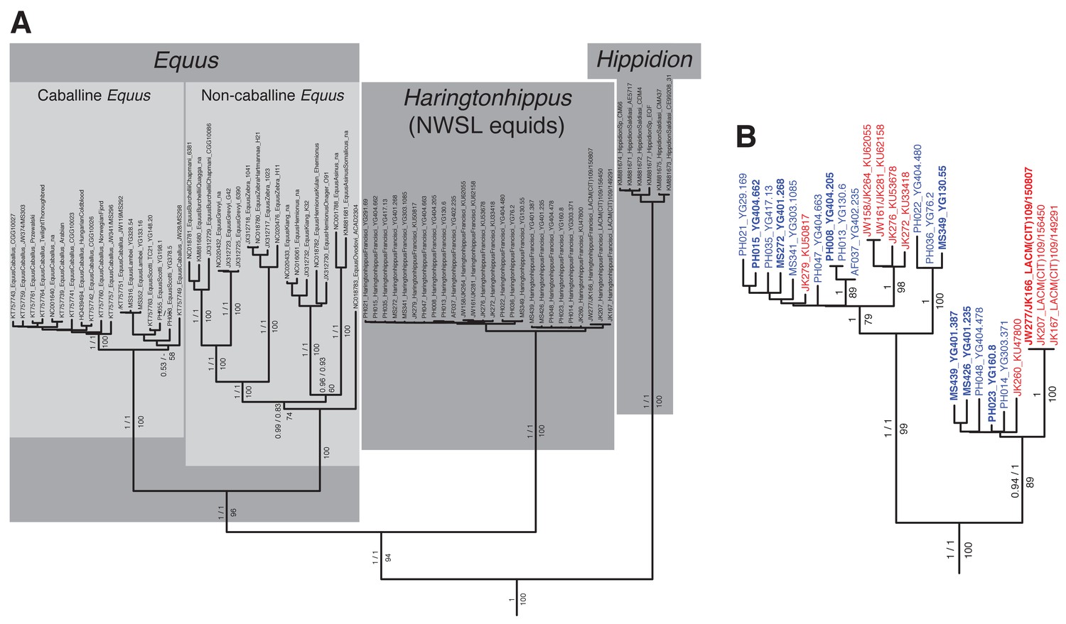
An example maximum likelihood (ML) phylogeny of equid mitochondrial genomes.
This topology resulted from the analysis of mtDNA data set 3 (see Appendix 1) with all partitions and Hippidion included, and dog and ceratomorphs as outgroup (not shown). Numbers above branches are Bayesian posterior probability support values from equivalent MrBayes and BEAST analyses, with those below indicating ML bootstrap values calculated in RAxML, and are shown for major nodes. (A) Full phylogeny of the analyzed equid sequences. (B) The Haringtonhippus (NWSL equid) clade, with tips color coded by geographic origin: east Beringia, blue; contiguous USA, red (following Figure 3). Tips in bold were included in the BEAST analysis (see also Supplementary file 1).
Figure 1—figure supplement 2
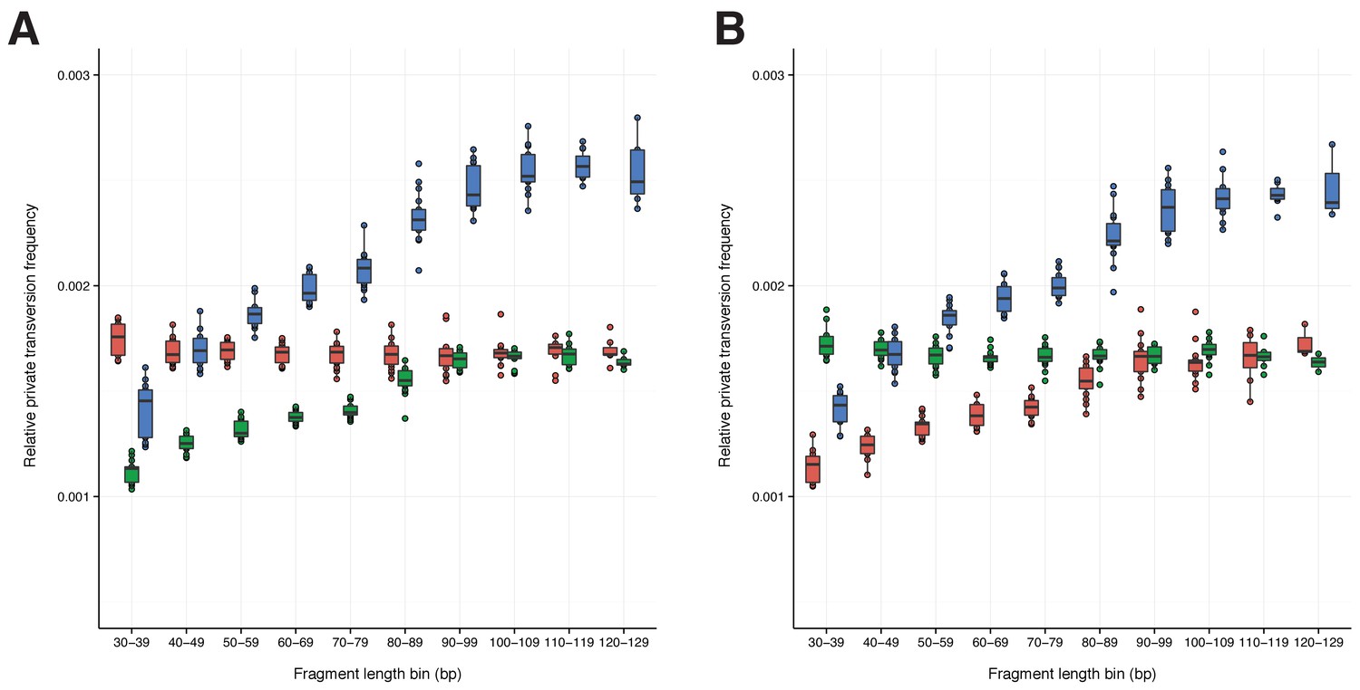
A comparison of relative private transversion frequencies between the nuclear genomes of a horse, donkey, and 17 NWSL equids.
A comparison of relative private transversion frequencies between the nuclear genomes of a caballine Equus (horse, E. caballus; green), a non-caballine Equus (donkey, E. asinus; red), and 17 NWSL equids (=Haringtonhippus francisci; blue) at different read lengths, with reads divided into 10 base pair (bp) bins. Analyses are based on alignment to the horse (A) or donkey (B) genome coordinates. To account for bins with low data content, we only display comparisons with at least 200,000 observable sites.
Figure 1—figure supplement 3

Calculation of divergence date estimates from nuclear genome data.
Relative branch lengths are from Figure 1—source data 3. Minimum (darker blue) and maximum (lighter blue) estimates are shown for the NWSL equid branch.
Figure 2 with 4 supplements

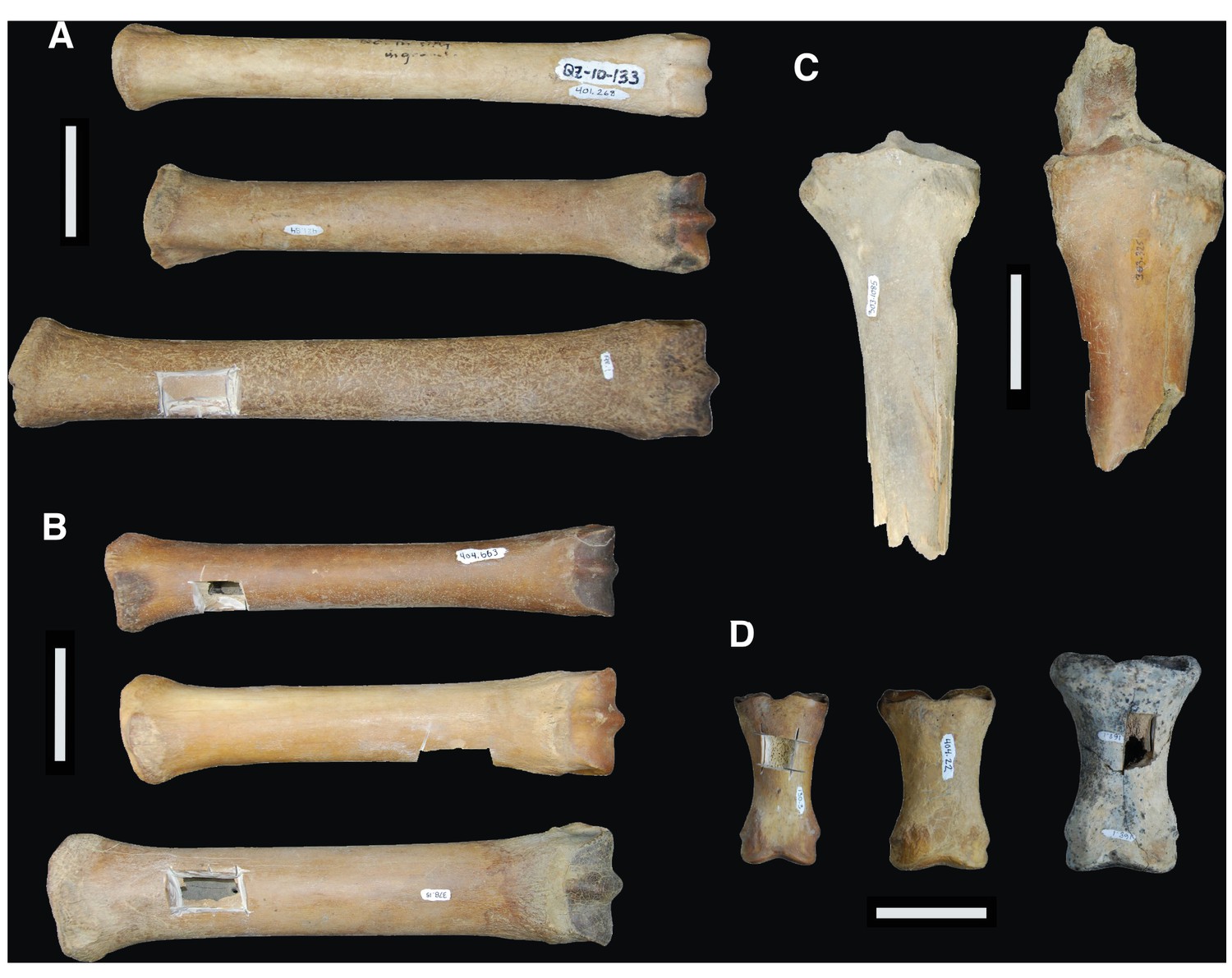
Morphological analysis of extant and middle-late Pleistocene equids.
(A) Crania of Haringtonhippus francisci, upper: LACM(CIT) 109/156450 from Nevada, lower: TMM 34–2518 from Texas. (B) From upper to lower, third metatarsals of: H. francisci (YG 401.268), E. lambei (YG 421.84), and E. cf. scotti (YG 198.1) from Yukon. Scale bar is 5 cm. (C) Principal component analysis of selected third metatarsals from extant and middle-late Pleistocene equids, showing clear clustering of stilt-legged (hemionine Equus (orange) and H. francisci (green)) from stout-legged (caballine Equus; blue) specimens (see also Figure 2—source data 1). Symbol shape denotes the specimen identification method (DNA: square, triangle: DNA/morphology, circle: morphology). The first and second principal components explain 95% of the variance.
-
Figure 2—source data 1
Measurement data for (A) equid third metatarsals, which were used in the morphometrics analysis, and (B) other NWSL equid elements.
- https://doi.org/10.7554/eLife.29944.015
Figure 2—figure supplement 1

The two crania assigned to H. francisci.
(A) LACM(CIT) 109/156450 from Nevada, identified through mitochondrial and nuclear palaeogenomic analysis. Upper: right side (reflected for comparison), lower: left side. (B) Part of the H. francisci holotype, TMM 34–2518 from Texas.
Figure 2—figure supplement 2
Comparison between the limb bones of H. francisci, E. lambei, and E. cf. scotti from Yukon.
(A) Third metatarsals from H. francisci (upper; YG 401.268), E. lambei (middle; YG 421.84), and E. cf. scotti (lower; YG 198.1). (B) Third metacarpals from H. francisci (upper; YG 404.663), E. lambei (middle; YG 109.6), and E. cf. scotti (lower; YG 378.15). (C) Proximal fragments of radii from H. francisci (left; YG 303.1085), and E. lambei (right; YG 303.325). (D) First phalanges from H. francisci (left; YG 130.3), E. lambei (middle; YG 404.22), and E. cf. scotti (right; YG 168.1).
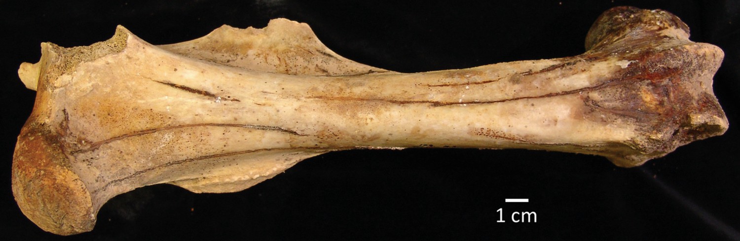
Figure 2—figure supplement 3
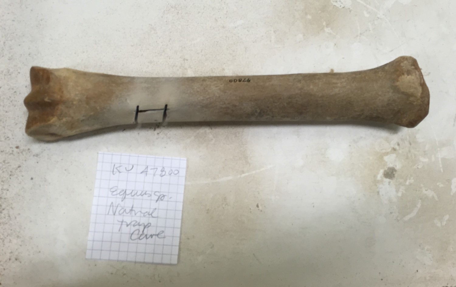
An example equid metacarpal from Natural Trap Cave, Wyoming.
This specimen (KU 47800; JK260) was originally referred to Equus sp., but is here identified as H. francisci on the basis of mitochondrial and nuclear genome data. We note the relative slenderness of this specimen, which is comparable to YG 404.663 (H. francisci) from Yukon in Figure 2—figure supplement 2.
Figure 2—figure supplement 4
An example femur of H. francisci from Gypsum Cave, Nevada.
This specimen (LACM(CIT)109/150708; JW277/JK166) was originally identified by Weinstock et al., 2005. List of Source data files.
Figure 3
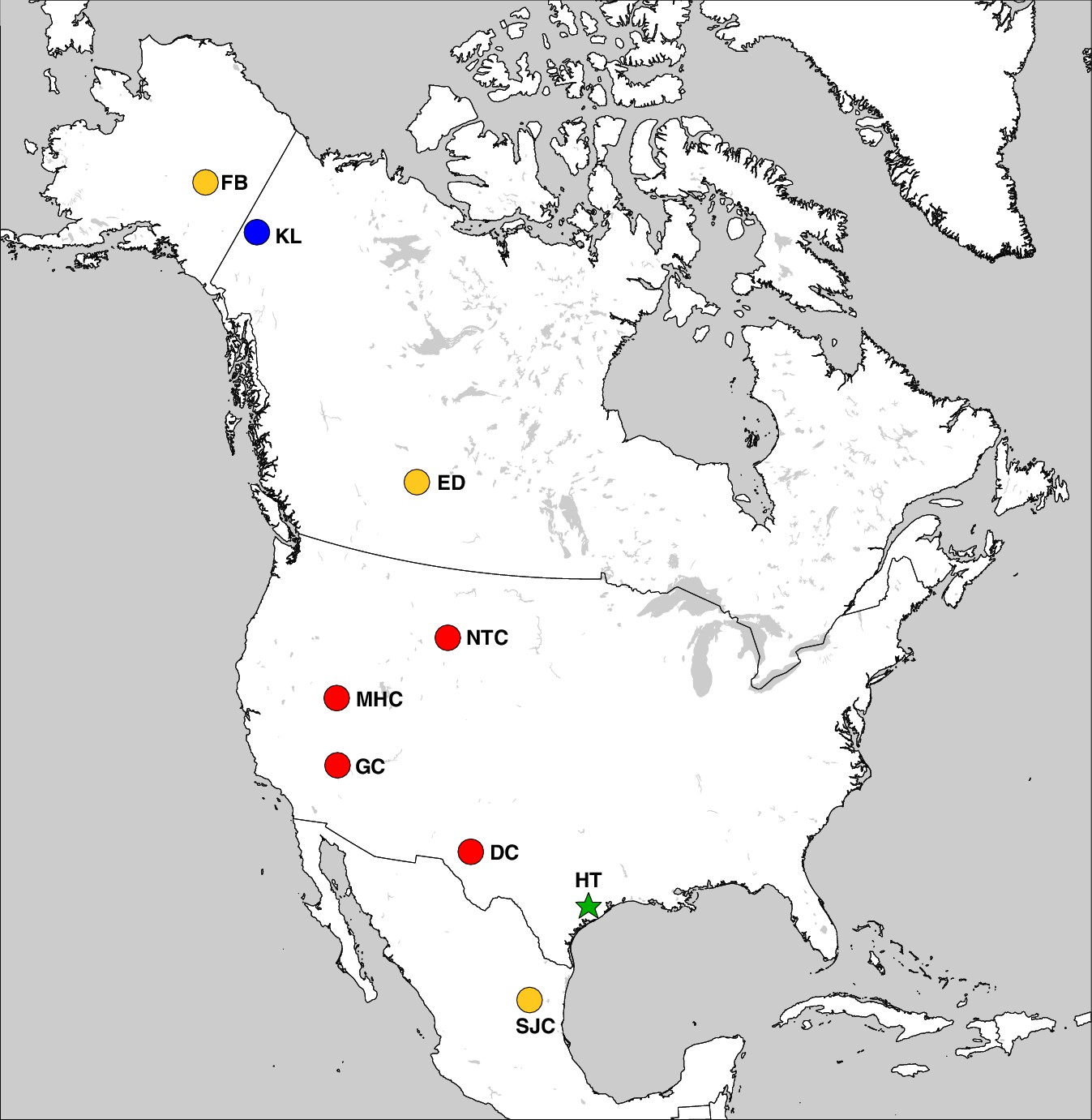
The geographic distribution of Haringtonhippus.
Blue circles are east Beringian localities (KL: Klondike region, Yukon Territory, Canada). Red circles are contiguous USA localities (NTC: Natural Trap Cave, Wyoming, USA; GC: Gypsum Cave, Nevada, USA; MHC: Mineral Hill Cave, Nevada, USA; DC: Dry Cave, New Mexico, USA [Barrón-Ortiz et al., 2017; Weinstock et al., 2005]). Orange circles are localities with tentatively assigned Haringtonhippus specimens only (FB: Fairbanks, Alaska, USA; ED: Edmonton, Alberta, Canada, USA; SJC: San Josecito Cave, Nuevo Leon, Mexico; (Barrón-Ortiz et al., 2017; Guthrie, 2003). The green-star-labeled HT is the locality of the francisci holotype, Wharton County, Texas, USA. This figure was drawn using Simplemappr (Shorthouse, 2010).
Appendix 1—figure 1
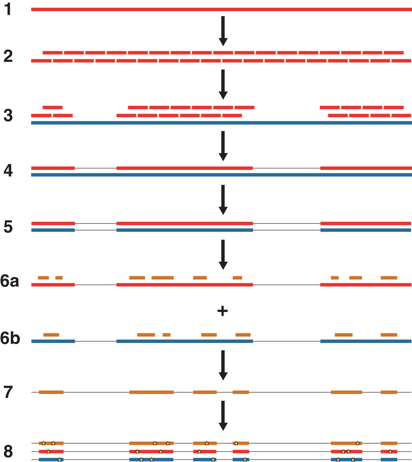
An overview of the nuclear genome analysis pipeline.
A first reference genome sequence (red; step 1) is divided into 150 bp pseudo-reads, tiled every 75 bp for exactly 2 × genomic coverage (step 2). These pseudo-reads are then mapped to a second reference genome (blue; step 3), and a consensus sequence of the mapped pseudo-reads is called (step 4). Regions of the second reference genome that are not covered by the pseudo-reads are masked (step 5). For each NWSL equid sample, reads (orange) are mapped independently to the first reference consensus sequence (step 6a) and masked second reference genome (step 6b). Alignments from steps 6a and 6b are then merged (step 7). For alignment coordinates that have base calls for the first reference, second reference, and NWSL equid sample genomes, the relative frequencies of private transversion substitutions (yellow stars) for each genome are calculated (step 8). The co-ordinates from the second reference genome (blue) are used for each analysis.
Appendix 2—figure 1
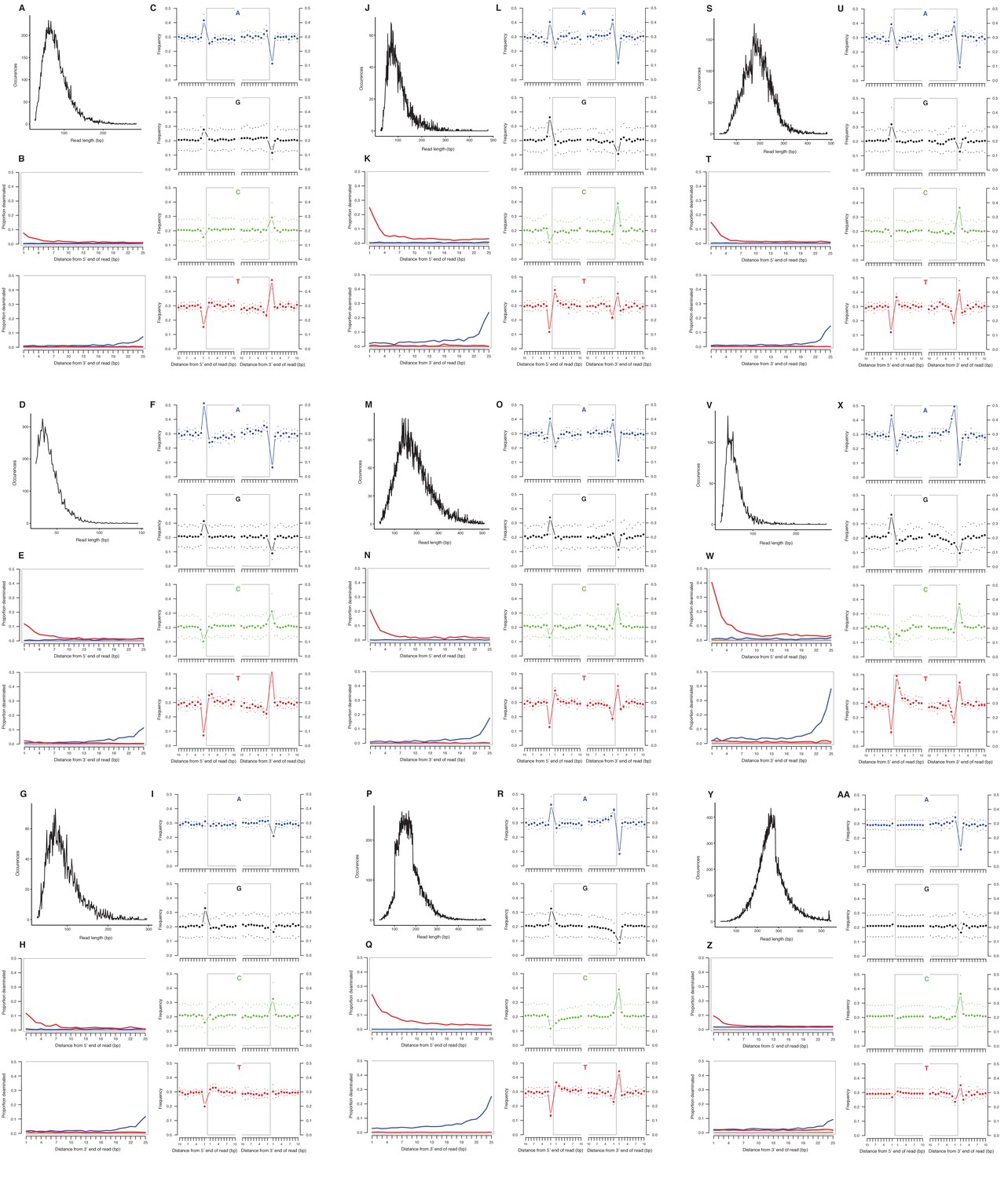
Characterization of ancient mitochondrial DNA damage patterns from nine equid samples.
H. francisci: (A–C) JK166 (LACM(CIT) 109/150807; Nevada), (D–F) JK207 (LACM(CIT) 109/156450; Nevada), (G–I) JK260 (KU 47800; Wyoming), (J–L) PH013 (YG 130.6; Yukon), (M–O) PH047 (YG 404.663; Yukon), (P–R) MS272 (YG 401.268; Yukon), (S–U) MS349 (YG 130.55; Yukon); E. cf. scotti: (V–X) PH055 (YG 198.1; Yukon); E. lambei: (Y–AA) MS316 (YG 328.54; Yukon). Every third panel: (A) to (Y) DNA fragment length distributions; (B) to (Z) proportion of cytosines that are deaminated at fragment ends (red: cytosine → thymine; blue: guanine → adenine); and (C) to (AA) mean base frequencies immediately upstream and downstream of the 5’ and 3’ ends of mapped reads.
Appendix 2—figure 2
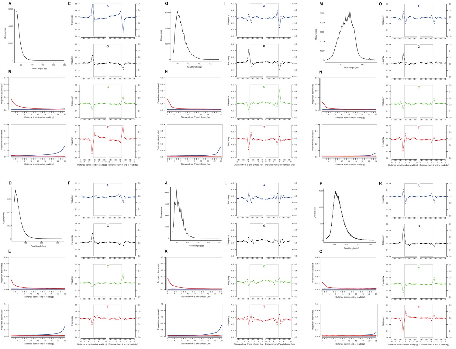
Characterization of ancient nuclear DNA damage patterns from six H. francisci samples.
(A–C) JK166 (LACM(CIT) 109/150807; Nevada), (D–F) JK260 (KU 47800; Wyoming), (G–I) PH013 (YG 130.6; Yukon), (J–L) PH036 (YG 76.2; Yukon), (M–O) MS349 (YG 130.55; Yukon), (P–R) MS439 (YG 401.387; Yukon). Every third panel: (A) to (P) DNA fragment length distributions; (B) to (Q) proportion of cytosines that are deaminated at fragment ends (red: cytosine → thymine; blue: guanine → adenine); and (C) to (R) mean base frequencies immediately upstream and downstream of the 5’ and 3’ ends of mapped reads.
Appendix 2—figure 3
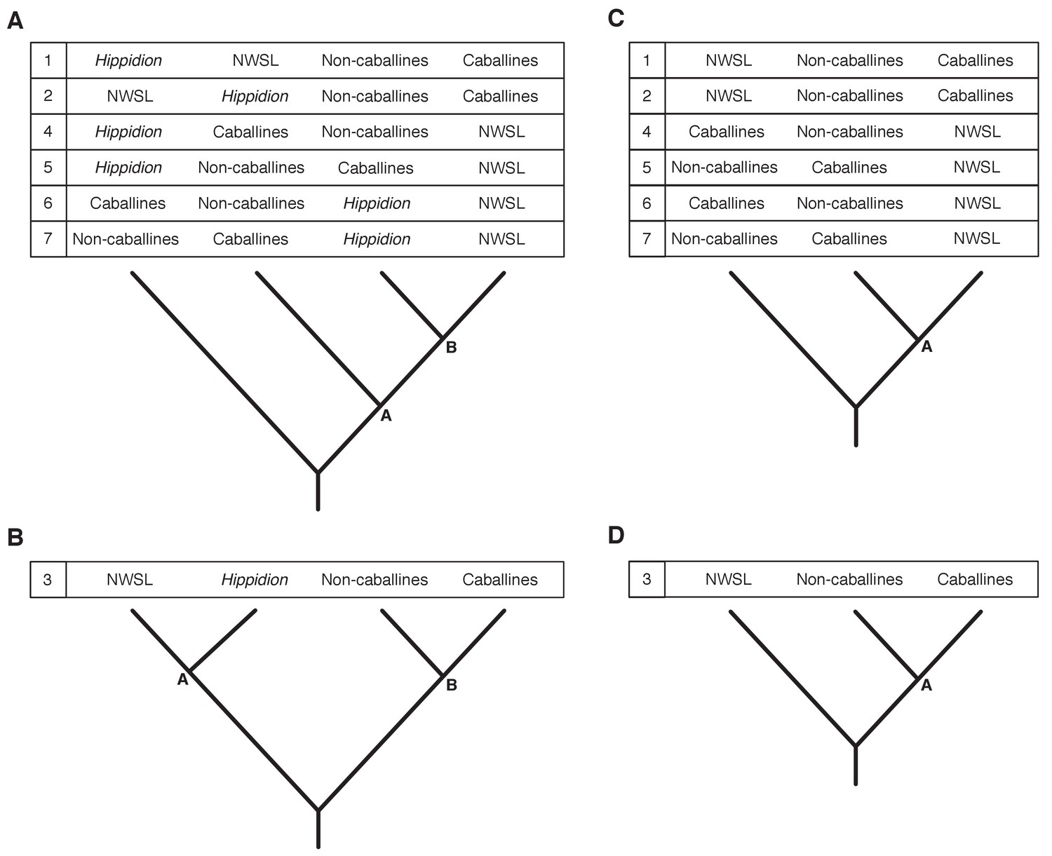
Seven phylogenetic hypotheses for the four major groups of equids with sequenced mitochondrial genomes.
These major groups are Hippidion, the New World stilt-legged equids (=Haringtonhippus), non-caballine Equus (asses, zebras, and E. ovodovi) and caballine Equus (horses). (A) imbalanced and (B) balanced hypotheses. The hypotheses presented in (C) and (D) are identical to (A) and (B), except that Hippidion is excluded. Node letters are referenced in Appendix 2—tables 1–2. We only list combinations that were recovered by our palaeogenomic, or previous palaeogenetic, analyses.
Appendix 2—figure 4
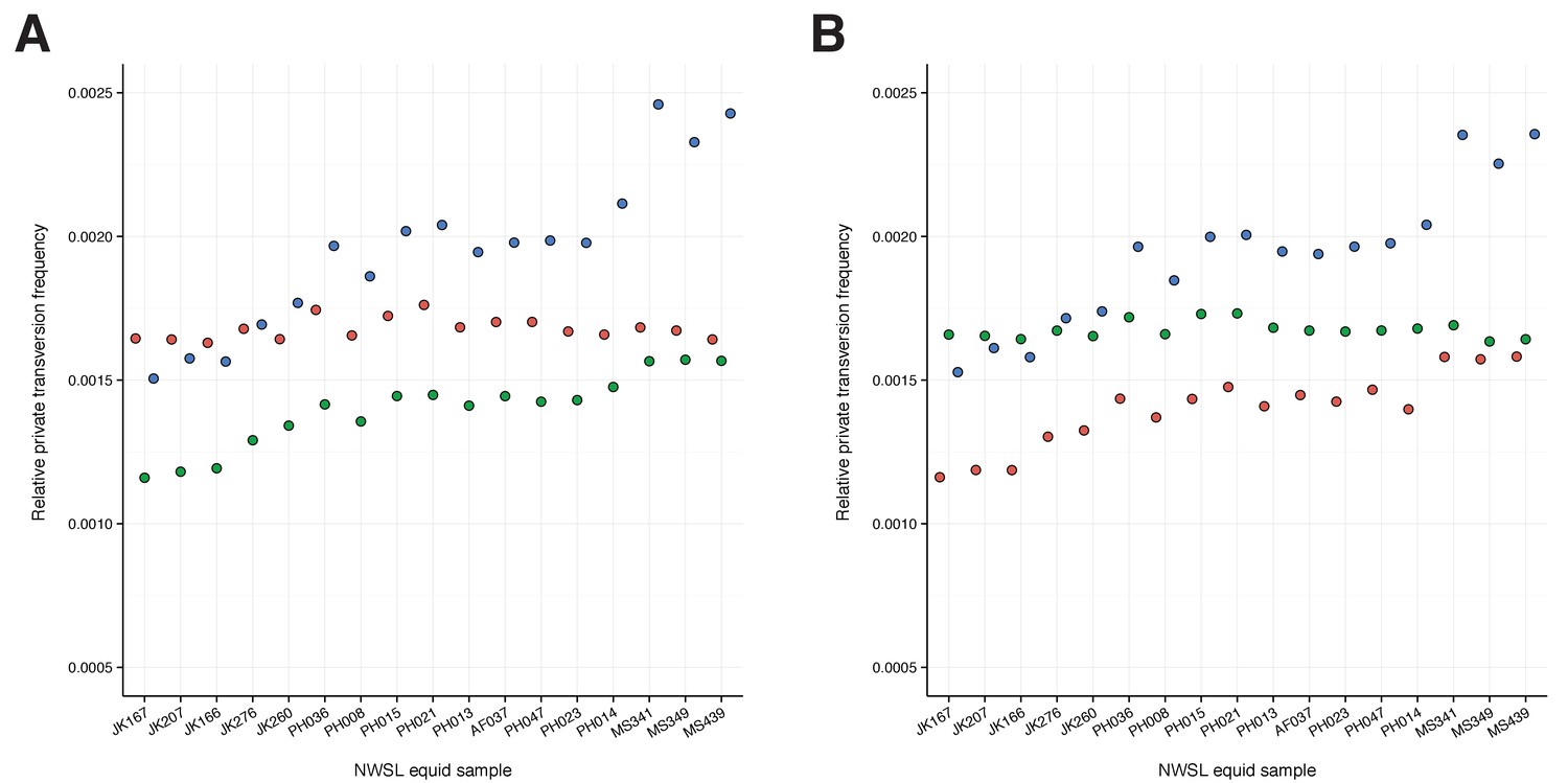
A comparison of relative private transversion frequencies between the nuclear genomes of a caballine Equus (horse, E.
caballus; green), a non-caballine Equus (donkey, E. asinus; red), and the 17 New World-stilt legged (NWSL) equid samples (=Haringtonhippus francisci; blue), using approach three (Appendix 1), with samples ordered by increasing mean mapped read length. Analyses are based on alignment to the horse (A) or donkey (B) genome coordinates.
Tables
Appendix 1—table 1
Selected models of molecular evolution for partitions of the first five mtDNA genome alignment data sets.
All lengths are in base pairs. Reduced length excludes the Coding3 and CR partitions. For all RAxML analyses the GTR model was implemented. *The TrN model was selected, but this cannot be implemented in MrBayes and so the HKY model was used. EPA: evolutionary placement algorithm; CR: control region.
| Data set | Partition | Total length | |||||||
|---|---|---|---|---|---|---|---|---|---|
| Coding1 | Coding2 | Coding3 | rRNAs | tRNAs | CR | All | Reduced | ||
| 1. White rhino outgroup | Length | 3803 | 3803 | 3803 | 2579 | 1529 | 1066 | 16583 | 11714 |
| Model | GTR + I + G | HKY + I + G | GTR + I + G | GTR + I + G | HKY + I + G | HKY*+I + G | |||
| 2. Malayan tapir outgroup | Length | 3803 | 3803 | 3803 | 2585 | 1530 | 1065 | 16589 | 11721 |
| Model | GTR + I + G | HKY + I + G | GTR + I + G | GTR + I + G | HKY + I + G | HKY*+G | |||
| 3. Dog + ceratomorphs outgroups | Length | 3803 | 3803 | 3803 | 2615 | 1540 | N/A | 15564 | 11761 |
| Model | GTR + I + G | HKY + I + G | GTR + I + G | GTR + I + G | HKY + I + G | N/A | |||
| 4. EPA | Length | 3803 | 3803 | 3803 | 2601 | 1534 | 1118 | 16662 | 11741 |
| Model | GTR + I + G | TrN + I + G | GTR + I + G | GTR + I + G | HKY + I + G | HKY + I + G | |||
| 5. Equids only | Length | 3802 | 3802 | 3802 | 2571 | 1528 | 971 | 16476 | 11703 |
| Model | TrN + I + G | TrN + I + G | GTR + G | TrN + I + G | HKY + I | HKY + G | |||
Appendix 1—table 2
Summary of the number and type of synapomorphic bases for each of the three examined equid genera.
A full list of these substitutions, and their position relative to the E. caballus reference mitochondrial genome (NC_001640), can be found in Appendix 1—table 2-Source data 1. *total includes a further five synapomorphic sites that have unique states in each genus.
| Substitution | Hippidion | Haringtonhippus | Equus |
|---|---|---|---|
| Transition | 338 | 147 | 66 |
| Transversion | 43 | 22 | 4 |
| Insertion | 2 | 4 | 0 |
| Deletion | 3 | 0 | 0 |
| Total* | 391 | 178 | 75 |
-
Appendix 1—table 2—source data 1
A compilation of all 634 putative synapomorphic sites in the mitochondrial genome for Hippidion, Haringtonhippus, and Equus (A), with a comparison to the published MS272 mitochondrial genome sequence at the 140 sites with a base state that matches one of the three genera (B).
The horse reference mtDNA has Genbank accession NC_001640.1.
- https://doi.org/10.7554/eLife.29944.022
Appendix 2—table 1
Topological shape and support values for the best supported trees.
These results are from the Bayesian and maximum likelihood (ML) analyses of mtDNA data sets 1–3, including either the all or reduced partition sets, and with Hippidion sequences either included or excluded. Topology numbers and node letters refer to those outlined in Appendix 2—figure 3. Bayesian posterior probability support of >0.99 and ML bootstrap support of >95% are in bold for nodes A and B. *support for nodes that are consistent with topology one in Appendix 2—figure 3. NCs: non-caballines.
| Outgroup | Partitions | Hippidion? | Tips | Analysis method | Topology | Support | |||||
|---|---|---|---|---|---|---|---|---|---|---|---|
| Node A | Node B | Hippidion | NWSL | NCs | Caballines | ||||||
| White rhino (Data set 1) | All | Excluded | 63 | Bayesian | 1/2/3 | 0.996* | N/A | N/A | 1.000 | 1.000 | 1.000 |
| ML | 1/2/3 | 71* | N/A | N/A | 100 | 99 | 100 | ||||
| Included | 69 | Bayesian | 2 | 0.751 | 1.000* | 1.000 | 1.000 | 1.000 | 1.000 | ||
| ML | 1 | 64* | 96* | 100 | 100 | 100 | 100 | ||||
| Reduced | Excluded | 63 | Bayesian | 1/2/3 | 1.000* | N/A | N/A | 1.000 | 1.000 | 1.000 | |
| ML | 1/2/3 | 100* | N/A | N/A | 99 | 100 | 100 | ||||
| Included | 69 | Bayesian | 2 | 0.948 | 1.000* | 1.000 | 1.000 | 1.000 | 1.000 | ||
| ML | 2 | 73 | 98* | 100 | 99 | 100 | 100 | ||||
| Malayan tapir (Data set 2) | All | Excluded | 63 | Bayesian | 5/7 | 0.971 | N/A | N/A | 1.000 | 1.000 | 1.000 |
| ML | 5/7 | 87 | N/A | N/A | 100 | 99 | 99 | ||||
| Included | 69 | Bayesian | 6 | 0.808 | 0.867 | 1.000 | 1.000 | 1.000 | 1.000 | ||
| ML | 6 | 55 | 63 | 100 | 100 | 100 | 100 | ||||
| Reduced | Excluded | 63 | Bayesian | 1/2/3 | 0.675* | N/A | N/A | 1.000 | 1.000 | 1.000 | |
| ML | 4/6 | 28 | N/A | N/A | 100 | 96 | 98 | ||||
| Included | 69 | Bayesian | 3 | 0.685 | 0.864* | 1.000 | 1.000 | 1.000 | 1.000 | ||
| ML | 3 | 70 | 69 | 100 | 100 | 100 | 100 | ||||
| Dog + ceratomorphs (Data set 3) | All | Excluded | 71 | Bayesian | 1/2/3 | 0.598* | N/A | N/A | 1.000 | 1.000 | 1.000 |
| ML | 4/6 | 59 | N/A | N/A | 100 | 100 | 100 | ||||
| Included | 77 | Bayesian | 1 | 1.000* | 1.000* | 1.000 | 1.000 | 1.000 | 1.000 | ||
| ML | 1 | 94* | 96* | 100 | 100 | 100 | 100 | ||||
| Reduced | Excluded | 71 | Bayesian | 1/2/3 | 0.999* | N/A | N/A | 1.000 | 1.000 | 1.000 | |
| ML | 1/2/3 | 97* | N/A | N/A | 100 | 100 | 100 | ||||
| Included | 77 | Bayesian | 1 | 1.000* | 1.000* | 1.000 | 1.000 | 1.000 | 1.000 | ||
| ML | 1 | 99* | 100* | 100 | 100 | 100 | 100 | ||||
Appendix 2—table 2
The a posteriori phylogenetic placement likelihood for eight ceratomorph (rhino and tapir) outgroups.
These analyses used a ML evolutionary placement algorithm, whilst varying the partition set used (all or reduced), and either including or excluding Hippidion sequences. Likelihoods >0.95 are in bold. Topology numbers refer to those outlined in Appendix 2—figure 3. Genbank accession numbers are given in parentheses after outgroup names.
| Partitions | Outgroup | Hippidion? | Included | Excluded | |||||
|---|---|---|---|---|---|---|---|---|---|
| Topology | 1 | 2 | 3 | 6 | 1/2/3 | 4/6 | 5/7 | ||
| All | Tapirus terrestris (AJ428947) | 0.456 | 0.317 | 0.205 | 0.018 | 0.549 | 0.313 | 0.139 | |
| Tapirus indicus (NC023838) | 0.275 | 0.105 | 0.225 | 0.389 | 0.050 | 0.908 | 0.042 | ||
| Coelodonta antiquitatis (NC012681) | 0.998 | 0.248 | 0.451 | 0.301 | |||||
| Dicerorhinus sumatrensis (NC012684) | 0.981 | 0.009 | 0.155 | 0.553 | 0.292 | ||||
| Rhinoceros unicornis (NC001779) | 0.998 | 0.529 | 0.334 | 0.137 | |||||
| Rhinoceros sondaicus (NC012683) | 0.989 | 0.006 | 0.732 | 0.196 | 0.072 | ||||
| Ceratotherium simum (NC001808) | 0.448 | 0.499 | 0.053 | 0.949 | 0.018 | 0.033 | |||
| Diceros bicornis (NC012682) | 0.917 | 0.065 | 0.018 | 0.851 | 0.073 | 0.076 | |||
| Reduced | Tapirus terrestris (AJ428947) | 0.410 | 0.391 | 0.199 | 0.987 | 0.012 | |||
| Tapirus indicus (NC023838) | 0.536 | 0.298 | 0.166 | 0.995 | |||||
| Coelodonta antiquitatis (NC012681) | 0.411 | 0.554 | 0.035 | 1.000 | |||||
| Dicerorhinus sumatrensis (NC012684) | 0.983 | 0.015 | 1.000 | ||||||
| Rhinoceros unicornis (NC001779) | 0.998 | 1.000 | |||||||
| Rhinoceros sondaicus (NC012683) | 0.895 | 0.102 | 1.000 | ||||||
| Ceratotherium simum (NC001808) | 0.296 | 0.704 | 1.000 | ||||||
| Diceros bicornis (NC012682) | 0.996 | 1.000 | |||||||
Appendix 2—table 3
The a posteriori phylogenetic placement likelihood for 21 published equid mitochondrial sequences.
These analyses used the ML evolutionary placement algorithm, whilst varying the partition set used (all or reduced), and either including or excluding Hippidion sequences. Sample names are given in parentheses after the species or group name. Localities are given for NWSL equids only. Likelihoods >0.95 are in bold. *Equus includes only caballines and non-caballine equids (NCE). **For EQ04 from Alberta, other placement likelihood values for the Hippidion included/excluded partitions were: Within caballines: 0.003/0.002, Sister to caballines: 0.002/0.002, Within NCE: 0.246/0.245, Sister to NCE: 0.004/0.003. No placements were returned for ‘within Hippidion’. bp: base pairs.
| Hippidion? | Partition | Published sample | Sequence length (bp) | Locality | Placement | |||||
|---|---|---|---|---|---|---|---|---|---|---|
| Sister to E. ovodovi | Sister to Hippidion | Within NWSL | Sister to NWSL | Sister to Equus* | Other** | |||||
| Included | All | E. ovodovi (ACAD2305) | 688 | 1.000 | ||||||
| E. ovodovi (ACAD2302) | 688 | 1.000 | ||||||||
| E. ovodovi (ACAD2303) | 688 | 1.000 | ||||||||
| H. devillei (ACAD3615) | 476 | N/A | 1.000 | |||||||
| H. devillei (ACAD3625) | 543 | N/A | 1.000 | |||||||
| H. devillei (ACAD3627) | 543 | N/A | 1.000 | |||||||
| H. devillei (ACAD3628) | 543 | N/A | 0.999 | |||||||
| H. devillei (ACAD3629) | 476 | N/A | 0.999 | |||||||
| NWSL equid (JW125) | 720 | Klondike, YT | N/A | 0.996 | ||||||
| NWSL equid (JW126) | 720 | Klondike, YT | N/A | 0.999 | ||||||
| Included | All | NWSL equid (EQ01) | 620 | Dry Cave, NM | N/A | 0.735 | 0.256 | |||
| NWSL equid (EQ03) | 117 | Dry Cave, NM | N/A | 0.002 | 0.974 | 0.011 | 0.003 | |||
| NWSL equid (EQ04) | 117 | Edmonton, AB | N/A | 0.004 | 0.703 | 0.014 | 0.007 | 0.255 | ||
| NWSL equid (EQ09) | 620 | Natural Trap Cave, WY | N/A | 0.981 | 0.014 | |||||
| NWSL equid (EQ13) | 620 | Natural Trap Cave, WY | N/A | 0.992 | ||||||
| NWSL equid (EQ16) | 464 | Dry Cave, NM | N/A | 0.854 | 0.138 | |||||
| NWSL equid (EQ22) | 620 | Natural Trap Cave, WY | N/A | 0.999 | ||||||
| NWSL equid (EQ30) | 393 | San Josecito Cave, MX-NL | N/A | 0.792 | 0.198 | |||||
| NWSL equid (EQ41) | 398 | Natural Trap Cave, WY | N/A | 0.997 | ||||||
| NWSL equid (JW328) | mitogenome | Mineral Hill Cave, NV | N/A | 1.000 | ||||||
| NWSL equid (MS272) | mitogenome | Klondike, YT | N/A | 1.000 | ||||||
| Reduced | NWSL equid (JW328) | mitogenome | Mineral Hill Cave, NV | N/A | 0.996 | |||||
| NWSL equid (MS272) | mitogenome | Klondike, YT | N/A | 1.000 | ||||||
| Excluded | All | E. ovodovi (ACAD2305) | 688 | 1.000 | N/A | N/A | ||||
| E. ovodovi (ACAD2302) | 688 | 1.000 | N/A | N/A | ||||||
| E. ovodovi (ACAD2303) | 688 | 1.000 | N/A | N/A | ||||||
| NWSL equid (JW125) | 720 | Klondike, YT | N/A | N/A | 0.996 | N/A | ||||
| NWSL equid (JW126) | 720 | Klondike, YT | N/A | N/A | 0.999 | N/A | ||||
| NWSL equid (EQ01) | 620 | Dry Cave, NM | N/A | N/A | 0.731 | 0.259 | N/A | |||
| NWSL equid (EQ03) | 117 | Dry Cave, NM | N/A | N/A | 0.980 | 0.010 | N/A | |||
| NWSL equid (EQ04) | 117 | Edmonton, AB | N/A | N/A | 0.721 | 0.013 | N/A | 0.252 | ||
| NWSL equid (EQ09) | 620 | Natural Trap Cave, WY | N/A | N/A | 0.987 | 0.008 | N/A | |||
| NWSL equid (EQ13) | 620 | Natural Trap Cave, WY | N/A | N/A | 0.993 | N/A | ||||
| NWSL equid (EQ16) | 464 | Dry Cave, NM | N/A | N/A | 0.844 | 0.148 | N/A | |||
| NWSL equid (EQ22) | 620 | Natural Trap Cave, WY | N/A | N/A | 0.999 | N/A | ||||
| NWSL equid (EQ30) | 393 | San Josecito Cave, MX-NL | N/A | N/A | 0.788 | 0.203 | N/A | |||
| NWSL equid (EQ41) | 398 | Natural Trap Cave, WY | N/A | N/A | 0.995 | N/A | ||||
| NWSL equid (JW328) | mitogenome | Mineral Hill Cave, NV | N/A | N/A | 1.000 | N/A | ||||
| NWSL equid (MS272) | mitogenome | Klondike, YT | N/A | N/A | 1.000 | N/A | ||||
| Reduced | NWSL equid (JW328) | mitogenome | Mineral Hill Cave, NV | N/A | N/A | 0.995 | N/A | |||
| NWSL equid (MS272) | mitogenome | Klondike, YT | N/A | N/A | 1.000 | N/A | ||||
Appendix 2—table 4
Sex determination analysis of 17 NWSL equids.
Chromosome ratio is the relative mapping frequency ratio between all autosomes and the X-chromosome. Males are inferred if the ratio is 0.45–0.55 and females if the ratio is 0.9–1.1.
| Sample | Museum accession | Chromosome ratio | Inferred sex |
|---|---|---|---|
| AF037 | YG 402.235 | 0.48 | male |
| JK166 | LACM(CIT) 109/150807 | 0.93 | female |
| JK167 | LACM(CIT) 109/149291 | 0.91 | female |
| JK207 | LACM(CIT) 109/156450 | 0.92 | female |
| JK260 | KU 47800 | 0.95 | female |
| JK276 | KU 53678 | 0.91 | female |
| MS341 | YG 303.1085 | 0.50 | male |
| MS349 | YG 130.55 | 0.48 | male |
| MS439 | YG 401.387 | 0.98 | female |
| PH008 | YG 404.205 | 0.90 | female |
| PH013 | YG 130.6 | 0.87 | probable female |
| PH014 | YG 303.371 | 0.46 | male |
| PH015 | YG 404.662 | 0.44 | probable male |
| PH021 | YG 29.169 | 0.83 | probable female |
| PH023 | YG 160.8 | 0.91 | female |
| PH036 | YG 76.2 | 0.81 | probable female |
| PH047 | YG 404.663 | 0.88 | probable female |
-
Appendix 2—table 4—source data 1
Data from the sex determination analyses of 17 NWSL equids, based on alignment to the horse genome (EquCab2).
- https://doi.org/10.7554/eLife.29944.033
Additional files
-
Supplementary file 1
Metadata for all samples used in the mitochondrial and nuclear genomic analyses, with the francisci holotype included for reference.
*mtDNA coverage is based on the iterative assembler or as previously published. **New mtDNA genome sequence, coverage, and radiocarbon data are reported for MS272.
- https://doi.org/10.7554/eLife.29944.017
-
Transparent reporting form
- https://doi.org/10.7554/eLife.29944.018
-
Appendix 1—table 2—source data 1
A compilation of all 634 putative synapomorphic sites in the mitochondrial genome for Hippidion, Haringtonhippus, and Equus (A), with a comparison to the published MS272 mitochondrial genome sequence at the 140 sites with a base state that matches one of the three genera (B).
The horse reference mtDNA has Genbank accession NC_001640.1.
- https://doi.org/10.7554/eLife.29944.022
-
Appendix 2—table 4—source data 1
Data from the sex determination analyses of 17 NWSL equids, based on alignment to the horse genome (EquCab2).
- https://doi.org/10.7554/eLife.29944.033
Download links
A two-part list of links to download the article, or parts of the article, in various formats.
Downloads (link to download the article as PDF)
Open citations (links to open the citations from this article in various online reference manager services)
Cite this article (links to download the citations from this article in formats compatible with various reference manager tools)
A new genus of horse from Pleistocene North America
eLife 6:e29944.
https://doi.org/10.7554/eLife.29944


