Tracking individual action potentials throughout mammalian axonal arbors
- ETH Zurich, Switzerland
Figures
Figure 1 with 1 supplement
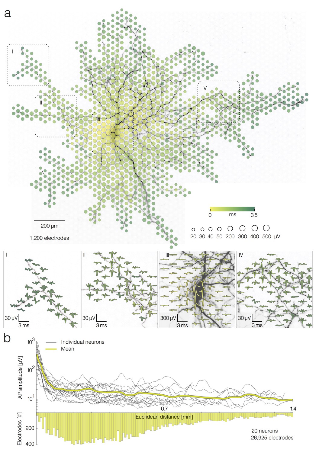
Average extracellular APs recorded neuron-wide.
(a) Extracellular AP footprint superimposed over neuronal morphology. Circle sizes indicate logarithmically scaled amplitudes of average APs obtained from 40 trials. Arrival time of the APs on different electrodes is color-coded. Close-ups of 4 regions (labeled I, II, III and IV), showing the average AP waveforms (40 trials), are presented at the lower part of (a). Individual APs recorded near the soma and axonal terminal are presented in Figure 2—figure supplement 1a. (b) AP amplitudes versus Euclidean distance from the footprint’s peak signal amplitude location for 20 neurons. Euclidean distance refers to the geometric distance between the electrode that recorded the largest-amplitude AP waveform (presumably at the AIS) and the respective recording electrode, it depends on the inter-electrode pitch. The yellow curve represents mean values of amplitudes over all neurons. The bottom histogram shows the distribution of electrode distances from the electrode that recorded the largest AP amplitude.
Figure 1—figure supplement 1
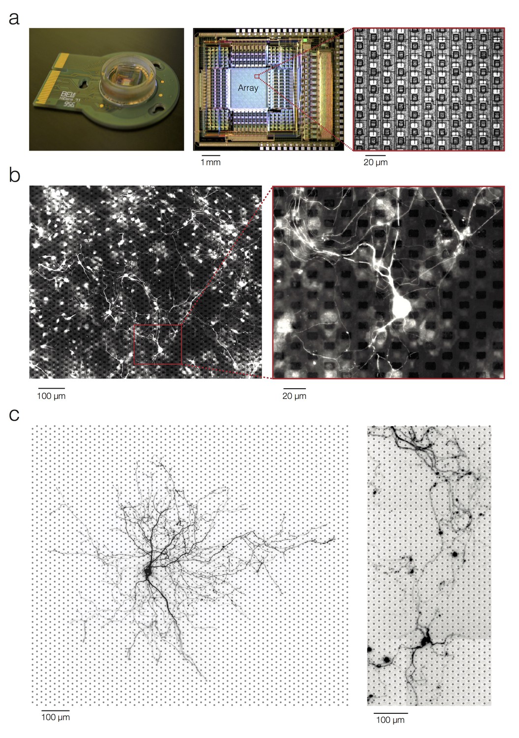
Experimental setup and preparation.
(a) CMOS –based high-density microelectrode array. (b) Micrograph of a rat primary neocortical culture grown on top of the HD-MEA. Immunostaining against Beta III Tubulin revealed neuronal processes. Microelectrodes can be seen as black or dark-grey squares in the background. The presented culture was fixed and stained on 15 DIV. 10,000 cells were plated. (c) Micrograph of rat primary neocortical neurons grown on top of the HD-MEA. Live imaging after, lipofection with red-fluorescent-protein DNA, revealed the morphology of individual neurons in the culture. Grey dots in the micrograph mark electrode locations. The neurons were lipofected on 12 DIV (left) and on 14 DIV (right). 20,000 cells in total were plated.
Figure 2 with 1 supplement
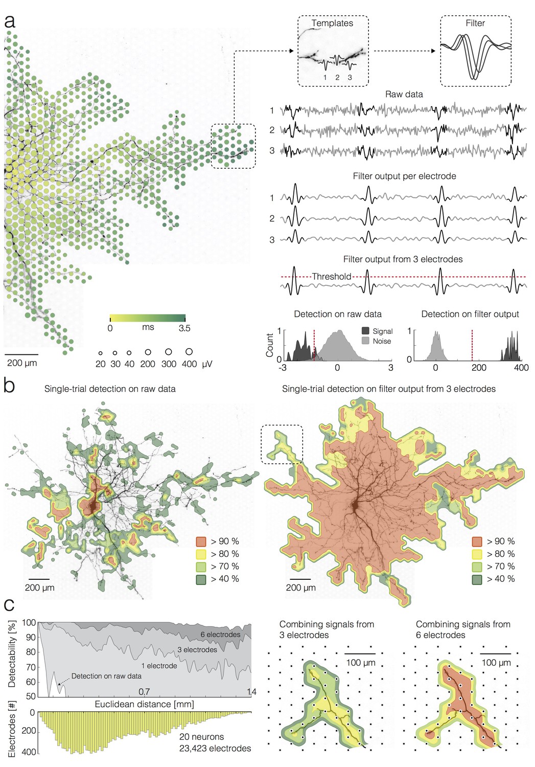
Detection of single APs on local groups of electrodes.
(a) (left) Extracellular AP footprint superimposed over neuronal morphology. Circle sizes and color code as in Figure 1(a). (right) AP templates recorded near the axonal terminal by three electrodes (denoted as 1, 2 and 3) and the corresponding AP detection filter are framed in boxes. Raw data recorded by the three electrodes (filter input), filter output per individual electrode, and filter output from the group of 3 electrodes are presented as light-gray traces. The AP detection threshold is presented by a red-dashed line. The detected signals are marked by dark-gray overlays on the raw data and filter outputs. Separability between signal and noise for the raw data (from the group of 3 electrodes) and for the filter output (from the group of 3 electrodes) are presented in histograms; distributions of signal and noise amplitudes are shaded in dark- and light-gray, respectively; the AP detection threshold is presented by the red-dashed line; the threshold was set to 5σnoise for simple-threshold detection, and the optimal threshold was computed for template-matching-based detection. (b) Detectability of single APs across the neuronal footprint is expressed as percentage of detected signals and presented through contoured surfaces. The obtained detectability is color-coded and superimposed over the neuronal morphology. (left) Signal detection applied on raw data. (right) Signal detection applied on the filter output from groups of 3 neighboring electrodes. (c) (left) Efficacy of single-AP detection (percentage of true positives) with respect to the number of electrodes, used to construct a filter (gray shades), and their Euclidean distance from the footprint’s peak signal amplitude location. Efficacy of the simple threshold-based detection applied to raw data is presented as a white surface in the graph. The bottom histogram shows the distribution of electrode distances from the electrode that recorded the largest AP waveform. (right) Improvement in AP detectability by increasing the number of electrodes to build the filter from 3 to 6. The close-up region is located in the upper left in Figure 2b (see marked box). Euclidean distance refers to the geometric distance between the electrode that recorded the largest-amplitude AP waveform and the respective recording electrode, it depends on the inter-electrode pitch.
Figure 2—figure supplement 1
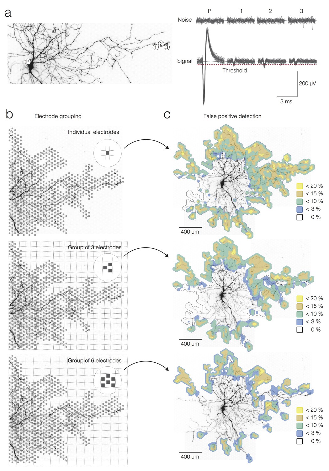
Ground truth, electrode-grouping and false-positive detections.
(a) (left) Positions of the recording sites with respect to the neuronal morphology. The white circle residing near the soma (denoted as ‘P’) is the position of the electrode that recorded large-amplitude signals during spontaneous activity used as a ground truth for single-trial detection in the axons. The white circles near an axonal terminal (denoted as 1, 2 and 3) represent electrodes that recorded signals used for single-trial detection. (right) Signal and noise of trials recorded from the four electrodes in (a). AP detection threshold (5σnoise) is presented by the red-dashed line. (b) Electrode-grouping approach used for template-matching-based detection. Grey squares represent electrodes that recorded signals for single-trial detection. Superimposed grids were used to cluster electrodes in local groups. The first panel shows no grouping; signals recorded by individual electrodes were used for the single-trial detection. Clustering in groups of 3 and 6 electrodes is shown in the second and third panel. (c) False-positive detection rate, expressed as a percentage of false-positives relative to the total number of detections per electrode, is color-coded and superimposed over the neuronal morphology for each electrode grouping in (b).
Figure 3
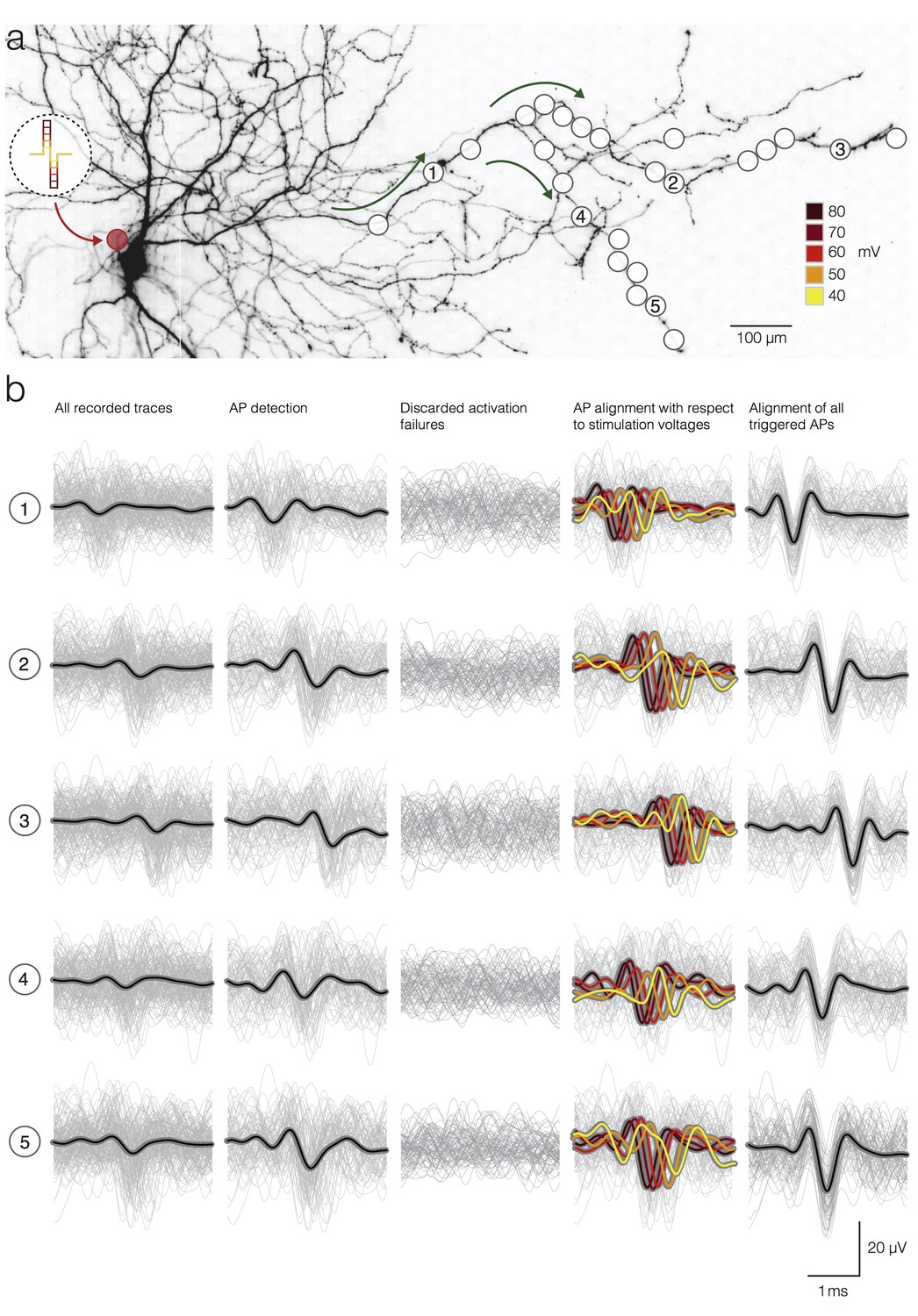
Detection and temporal alignment of axonal APs triggered by stimulation.
(a) Positions of stimulation and recording sites with respect to the neuronal morphology. The red circle near the soma represents the position of the stimulation electrode; white circles mark recording electrodes below axonal branches. Green arrows denote the direction of AP propagation. The biphasic voltage pulses used to stimulate the neuron are depicted within the circular inset. The voltage magnitudes are color-coded. Signals recorded by 5 electrodes (labeled as 1, 2, 3, 4 and 5) are presented below in (b). (b) Stimulation-triggered recorded by the 5 marked electrodes in (a) are presented in rows. The columns indicate different stages of the detection process. Average signals are represented by black lines; single trials are represented by gray traces. The first column shows all recorded traces, even those, where no action potential was elicited by the stimulation, temporally aligned on the stimulation onset. The second column shows only the detected APs. The third column shows the discarded activation failures. The fourth column shows detected APs; APs were grouped, and their average waveforms were color-coded according to the magnitudes of the stimulation voltage. The fifth column shows the detected APs aligned according to the time of AP occurrence at the respective electrodes taking into account the respective activation latencies.
Figure 4

Activation latencies and AP propagation jitter.
(a–d) Dependence of the activation latency and activation precision on the stimulation voltage. (a) Experimental design: the red circle denotes the position of the stimulation electrode; the white circle denotes the position of a recording electrode; the red arrow indicates the direction of AP propagation. (b) Excitability profile of the neuron shown in (a): the stimulation threshold, sub-threshold, intermediary and supra-threshold regimes are indicated in the graph. (c) Decrease in activation latency upon increasing the stimulation voltage: activation latencies obtained from eight neurons are represented by dark-gray curves; mean activation latency is presented by the yellow curve; the stimulation voltage has been normalized with respect to the stimulation threshold (threshold voltage was set to one); the widths of the intermediary regimes of 8 neurons are presented by dark-gray lines in the upper-right corner. (d) Decrease in activation jitter with increasing stimulation voltage; activation jitters obtained from eight neurons are represented by dark-gray curves; the average activation jitter is represented by the yellow curve. (e–h) Increase in the AP propagation jitter with axial distance along the axon. Axial distances were measured along the studied axonal branches; they also depend on the inter-electrode pitch. (e) Two axonal branches are labeled (‘Branch 1’ and ‘Branch 2’) and marked by a dark-green and a light-green line, respectively. White circles indicate the positions of the recording electrodes. (f) AP propagation times obtained from the two branches: average propagation times are presented by solid lines; the standard deviations of the propagation times are represented by pale bands in the background. (g) APs captured near four axonal sites that correspond to the electrodes labeled as 1–4 in (e): the recorded signals were aligned with respect to the AP arrival time detected on electrode 1; the peaks of individual APs (10 APs per electrode) were magnified and projected onto a raster and box-and-whisker plot. (h) Increase in the standard deviation (std) of the AP propagation jitter with axial distance from the first detection site near the soma: the AP propagation jitters, obtained from six neurons, are represented by dark-gray circles; the fitted yellow line was obtained by linear regression of the variance of the arrival times against axial distance. The histogram shows the distribution of electrode distances from the location of the first action potential detection.
Figure 5
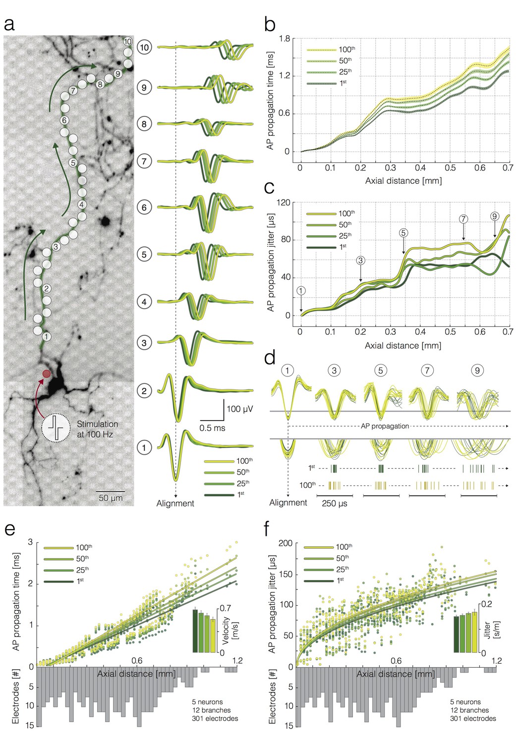
Activation-frequency-dependent changes in AP propagation times and jitters.
(a) (left) Position of stimulation and recording sites with respect to the neuronal morphology. The red circle represents the stimulation electrode; the white circles mark recording electrodes along an axon. Biphasic voltage pulses, used to stimulate the neuron, are depicted within the circular inset. The neuron was stimulated 100 times with 100 pulses at 100 Hz. Signals recorded by 10 electrodes (labeled as 1–10) are presented at the right. (right) Average APs recorded by the labeled electrodes were aligned with respect to the arrival time of the signal detected on electrode 1. Average APs, triggered by the 1st, 25th, 50th and 100th stimulation pulse, are color coded. (b) Propagation times of APs triggered by the 1st, 25th, 50th and 100th stimulation: average propagation times are presented as black dashed lines; standard errors (SEM) are color-coded and represented by pale bands. The data were obtained from the neuron shown in (a). (c) AP propagation jitters, observed during neuronal response to the 1st, 25th, 50th and 100th stimulation, are represented through color-coded curves. The data were obtained from the neuron shown in (a). (d) Individual AP trials, triggered by the 1st and 100th stimulation are colored in green and yellow; the APs were recorded near 5 axonal sites (labeled as 1, 3, 5, 7 and 9) that correspond to the sites marked in (a, c); the recorded signals were aligned with respect to the arrival time of APs detected on electrode 1; aligned signals, triggered by the 1st and 100th stimulation pulse, were superimposed and centered with respect to occurrence time for the sake of comparison; the peaks of individual APs` were magnified and projected onto raster plots. Note the differences in the jitter of AP trials triggered by the 1st and 100th stimulation pulse. (e) Deceleration of AP propagation during high-frequency stimulation: the average AP propagation times, observed during neuronal response to the 1st, 25th, 50th and 100th stimulation pulse, are presented through color-coded circles; the data obtained from four neurons (12 axonal branches in total) are jointly displayed; fitted lines were obtained by using linear regression. Inset: the color-coded histogram shows AP propagation velocities during neuronal response to the 1st, 25th, 50th and 100th stimulation pulse; the values were calculated from the slope of the linear regression. (f) Increase in AP propagation jitter during high-frequency stimulation: the AP propagation jitter, observed during neuronal response to the 1st, 25th, 50th and 100th stimulation, are presented through color-coded circles; the data obtained from four neurons (12 axonal branches in total) are jointly displayed; the fitted lines were obtained using linear regression of the variance of the arrival times against axial distance. Inset: the color-coded histogram shows the propagation jitter observed during neuronal response to the 1st, 25th, 50th and 100th stimulation; the values were calculated from the square root of the slope of the linear regression. Axial distances in (b), (c), (e) and (f) were measured along the specific observed axonal branch with all its turns; they are also depending on the electrode pitch (17.8 µm center-to-center pitch).
Author response image 1

Amplitude variability as a function of stimulation number.
The plot shows the standard deviation of the spike amplitudes of the neuron shown in Figure 5 of the main text as a function of stimulation number (1st to 100th). The standard deviation is computed over 39 repetitions for each individual electrode (grey lines). The black line shows the mean over all electrodes; the green line the linear regression to the mean. The average standard deviation of amplitudes for periods of noise is shown in red as a comparison. The average standard deviation of spike amplitudes increases with stimulation number (7% from 1st stimulation to 100th stimulation), but the increase is small.
Author response image 2
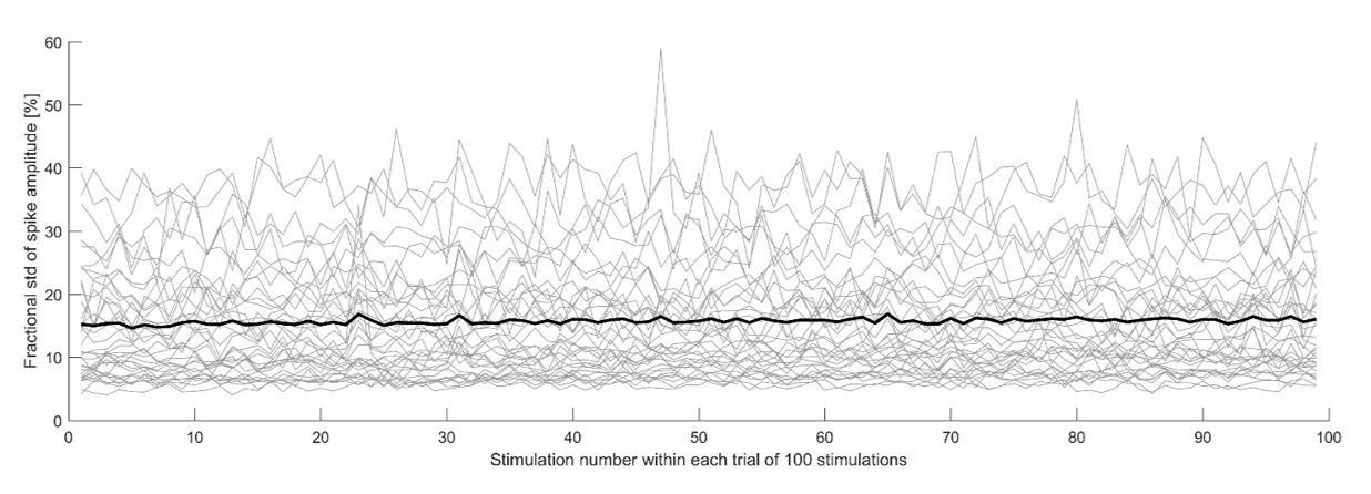
Fractionalamplitude variability as a function of stimulation number.
The plot shows the standard deviation of the spike amplitude, divided by the spike amplitude for each electrode, of the neuron shown in Figure 5 of the main text.
Additional files
-
Transparent reporting form
- https://doi.org/10.7554/eLife.30198.009
Download links
A two-part list of links to download the article, or parts of the article, in various formats.
Downloads (link to download the article as PDF)
Open citations (links to open the citations from this article in various online reference manager services)
Cite this article (links to download the citations from this article in formats compatible with various reference manager tools)
Tracking individual action potentials throughout mammalian axonal arbors
eLife 6:e30198.
https://doi.org/10.7554/eLife.30198


