Figures and data in Evolutionary dynamics of incubation periods

Figures
Tables
Additional files

9 figures, 1 table and 2 additional files

Figures

Figure 1

Download asset Open asset

Frequency distributions of incubation periods for two diseases.

Data redrawn from historic examples. Dashed red curves are noncentral lognormal distributions. Solid blue curves are Gumbel distributions, predicted by the theory developed here. Both sets of curves were fitted via the method of moments. (a) Data from an outbreak of food-borne streptococcal sore throat, reported in 1950 (Sartwell, 1950). Time is measured in units of days. (b) Data from a 1949 study of bladder tumors among workers following occupational exposure to a carcinogen in a dye plant (Goldblatt, 1949). Time is measured in units of years.

https://doi.org/10.7554/eLife.30212.003

Figure 2

Download asset Open asset

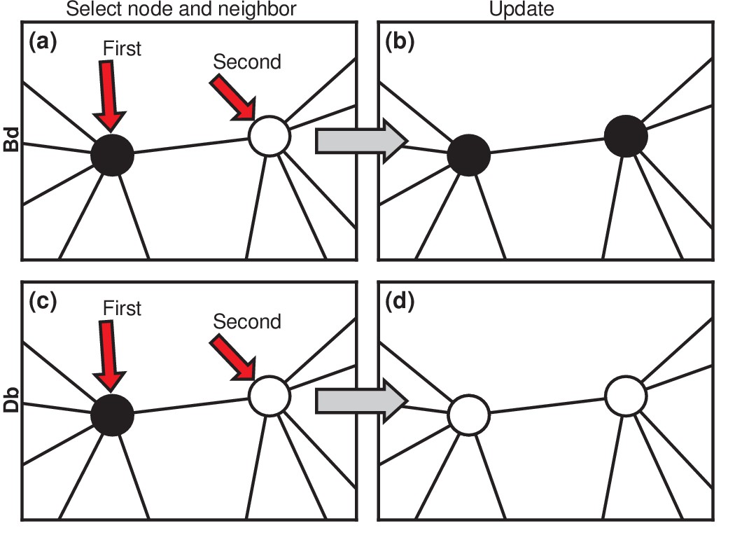
Evolutionary update rules.

(a) In the Birth-death (Bd) update rule, a node anywhere in the network is selected at random, with probability proportional to its fitness, and one of its neighbors is selected at random, uniformly. (b) The neighbor takes on the type of the first node. In biological terms, one can interpret this rule in two ways: either the first node transforms the second; or it gives birth to an identical offspring that replaces the second. (c) In the Death-birth (Db) update rule, a node is selected at random to die, with probability inversely proportional to its fitness, and one of its neighbors is selected at random, uniformly, to give birth to one offspring. (d) The first node is replaced by the offspring of the second.

https://doi.org/10.7554/eLife.30212.005

Figure 3

Download asset Open asset

Network topology and invader fitness shape the distribution of incubation periods.

Plots show simulated distributions of incubation periods, defined here as invader fixation times. Starting from a single invader at a random node, the state of the network was updated by Birth-death dynamics on both a complete graph and a two-dimensional (2D) lattice. Results for the Death-birth update rule (not shown) are identical. All distributions are normalized to have zero mean and unit variance. (a) Infinitely fit invader. For invader fitness $r \to \infty$ , the distribution is right-skewed for a complete graph (blue symbols). It approaches a Gumbel distribution as $N \to \infty$ , where $N$ is the number of nodes in the network. In contrast, for a 2D lattice (red symbols) the incubation periods are normally distributed. The difference is that a coupon collection mechanism operates in the complete graph and in lattices of sufficiently high dimension $d \geq 3$ ; this mechanism causes the right skew. Simulations used $10^{6}$ repetitions on a complete graph of $N = 150$ nodes, and $10^{5}$ repetitions for a 2D lattice of $N = 30^{2}$ nodes. (b) Neutrally fit invader. Distributions of incubation periods are shown for invader fitness $r = 1$ , using $10^{6}$ repetitions on a complete graph of $N = 50$ nodes (blue symbols), and $10^{5}$ repetitions for a 2D lattice of $N = 7^{2}$ nodes (red symbols). Similar right-skewed distributions occur for both networks, caused by a conditioned random walk mechanism.

https://doi.org/10.7554/eLife.30212.007

Figure 4

Download asset Open asset

Testing robustness.

The plots show how the distribution of incubation periods does or does not change when we modify the assumed update rules and criterion for the onset of symptoms. Both Birth-death (Bd) and Death-birth (Db) dynamics were simulated on a complete graph of $N = 5000$ nodes, using a infinite invader fitness. Incubation periods are now defined as times needed for invaders to take over a fraction $f$ of the whole network. All distributions are normalized to have zero mean and unit variance. Data points are color-coded according to the nature of the distribution: blue indicates a Gumbel distribution, and red indicates a normal distribution. (a) The distribution of times till invader fixation ( $f = 1$ ) under Birth-death dynamics. The Gumbel distribution of Figure 3a persists. (b) When $f$ is reduced to 0.9, the incubation periods under Birth-death dynamics become normally distributed instead of skewed. (c) When $f$ is reduced to 0.1, the incubation period distribution remains normally distributed. By contrast, Death-birth dynamics are insensitive to this modification: the Gumbel distribution persists not only for (d) $f = 1$ but even for (e) $f = 0.9$ and (f) $f = 0.1$ . The difference in sensitivity between the two types of dynamics can be explained intuitively by when the slowest part of the coupon collection process occurs. For Death-birth dynamics, it occurs near the *beginning* of the invasion, when it takes a long time to randomly select one of the few available invaders to give birth. Since the slow part of coupon collection occurs near the beginning, it is insensitive to the end-condition $f < 1$ . In contrast, the slow part occurs near the *end* of the invasion for Birth-death dynamics (when residents are scarce), and hence gets truncated when $f < 1$ , giving rise to a normal instead of a right-skewed distribution.

https://doi.org/10.7554/eLife.30212.008

Figure 5

Download asset Open asset

Robustness to heterogeneity.

Simulated, fitted, and normalized distributions of incubation periods for birth-death dynamics on a complete graph of $N = 500$ nodes. Unless stated otherwise, each simulation used an invader fitness of $r = 10$ , measured times till complete takeover ( $f = 1$ ), and started from an initial dose of 1 invader. Runs where the dosage was not smaller than the truncation point were rejected. The blue curves indicate noncentral lognormals fitted via the method of moments. (a) Heterogeneous fitness of invader. Every run used a different $r$ selected from a Gamma distribution with a shape parameter of 10. (b) Heterogeneity of host response. Instead of waiting until all $N$ residents had been replaced by invaders, every run used a different truncation point uniformly selected from ${2, 3, \dots N}$ . (c) Heterogeneity of dosage. Every run had a different starting population drawn from a Poisson of mean 10 and a shift of 1. (d) Heterogeneity of invader fitness, host response, and dosage. Every run used an $r$ drawn from Gamma(10), a truncation point $f$ drawn from Uniform(0,1), and a dosage drawn from Poisson(10)+1.

https://doi.org/10.7554/eLife.30212.009

Figure 6

Download asset Open asset

Network dependence of incubation periods.

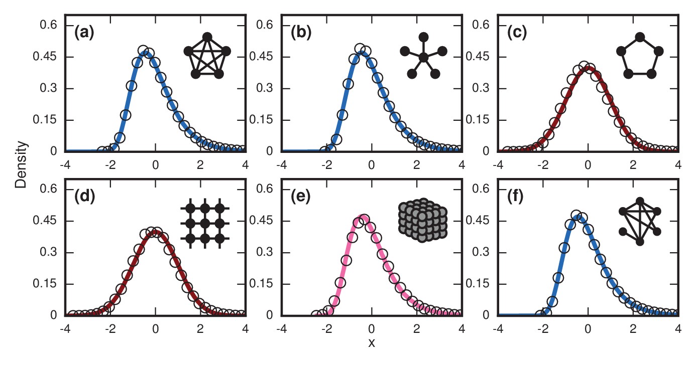
Distributions of invader fixation times, normalized to have zero mean and unit variance, are shown for infinite- $r$ Birth-death dynamics on various networks. Open circles show simulation results. Curves show analytical predictions: blue curves are Gumbels, red are normals, and pink is an intermediate distribution. Insets show schematics of networks. (a) The distribution of fixation times for a complete graph on $N = 150$ nodes, for $10^{6}$ runs. Distribution normalized according to analytically calculated mean and standard deviation. Curve shows a Gumbel distribution. (b) The Gumbel distribution of fixation times for a star graph with $N = 75$ spokes, for $10^{6}$ runs. Distribution normalized according to analytically calculated mean and standard deviation. (c) Normal distribution of fixation times for a 1D ring on $N = 75$ nodes, for $10^{6}$ runs. Distribution normalized according to analytically calculated mean and standard deviation. (d) Normal distribution of fixation times for a 2D lattice of $N = 60 \times 60$ nodes, for $10^{5}$ runs. Distribution normalized according to empirically calculated mean and standard deviation. (e) The distribution of fixation times for a 3D lattice of $N = 11^{3}$ nodes, for $10^{5}$ runs. Distribution normalized according to empirically calculated mean and standard deviation. The predicted distribution is the result of an approximating sum of exponential random variables under $10^{6}$ repetitions. (f) The distribution of fixation times for an Erdős-Rényi random graph on $N = 115$ nodes with an edge probability of $ρ = 0.5$ . Distribution normalized according to empirically calculated mean and standard deviation.

https://doi.org/10.7554/eLife.30212.011

Figure 7

Download asset Open asset

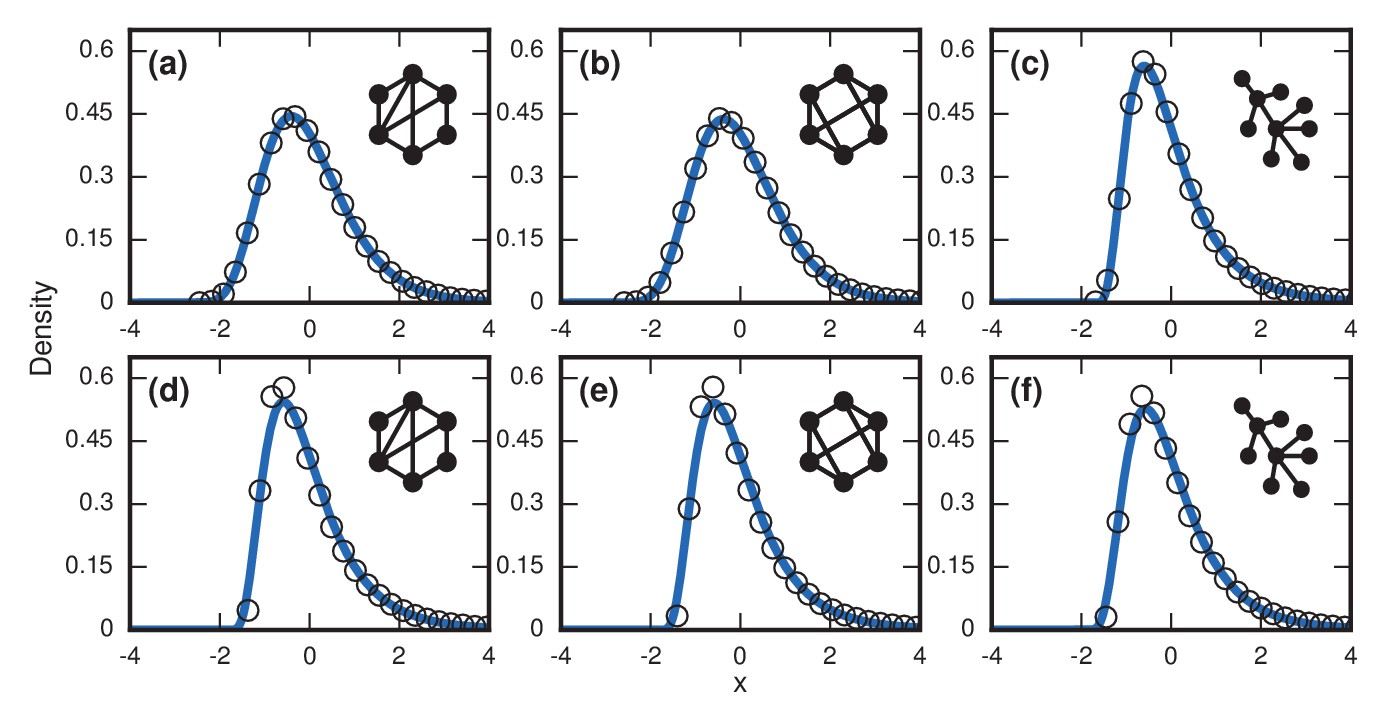
Complex networks.

Simulated and fitted distributions of invader fixation times for Birth-death dynamics on small-world, scale-free, and $k$ -regular networks. All distributions were normalized to have mean zero and unit variance. The curves indicate non-central lognormals fitted to the first three moments of the data. All distributions are the result of $10^{6}$ simulations. The figures in the top row ((a), (b), (c)) used invader fitness $r = \infty$ , whereas the figures in the bottom row ((d), (e), (f)) used neutral fitness $r = 1$ . (a) Newman-Watts-Strogatz small-world ring network with shortcut probability of $ρ = 0.25$ on $N = 75$ . (b) Random 3-regular graph on $N = 100$ nodes. (c) Barabasi-Albert scale-free network with a minimum degree of 3 and $N = 100$ nodes. (d) Newman-Watts-Strogatz small-world ring network with shortcut probability of $ρ = 0.25$ on $N = 25$ nodes. (e) Random 3-regular graph on $N = 22$ nodes. (f) Barabasi-Albert scale-free network with a minimum degree of 3 and $N = 22$ nodes.

https://doi.org/10.7554/eLife.30212.012

Figure 8

Download asset Open asset

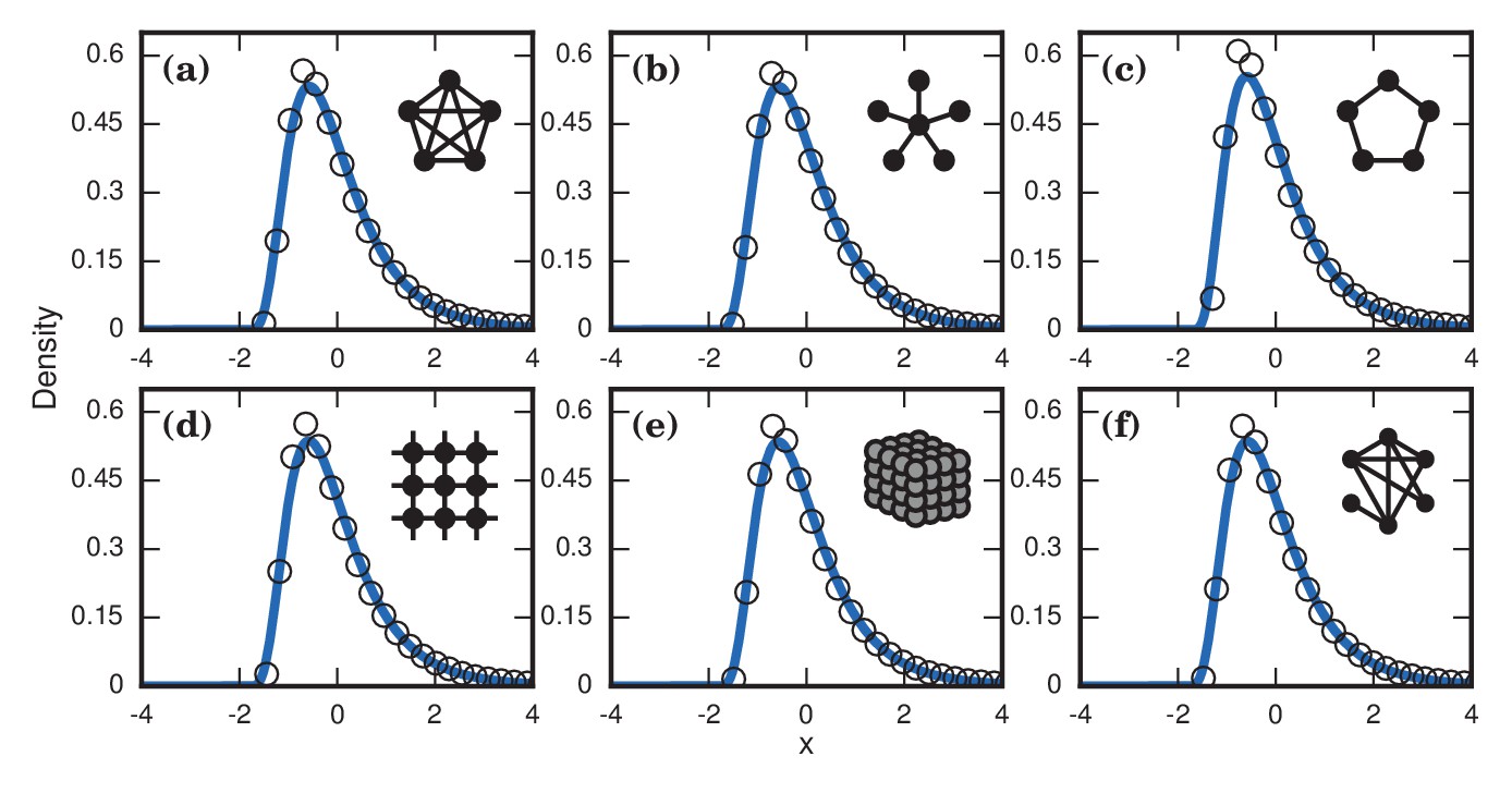
Neutrally fit invader $(r = 1)$ .

Simulated and fitted distributions of invader fixation times are shown for Birth-death dynamics on various networks. All distributions were normalized to have mean zero and unit variance. The curves indicate noncentral lognormals fitted via the method of moments. (a) Complete graph on $N = 50$ nodes, for $10^{6}$ runs. (b) Star graph with $N = 25$ spokes, for $10^{6}$ runs. (c) One-dimensional ring on $N = 50$ nodes, for $10^{6}$ runs. (d) Two-dimensional lattice on $N = 7 \times 7$ nodes, for $10^{6}$ runs. (e) Three-dimensional lattice on $N = 4^{3}$ nodes for $10^{6}$ runs. (f) Erdős-Rényi random graph on $N = 25$ nodes with an edge probability of $ρ = 0.5$ .

https://doi.org/10.7554/eLife.30212.013

Figure 9

Download asset Open asset

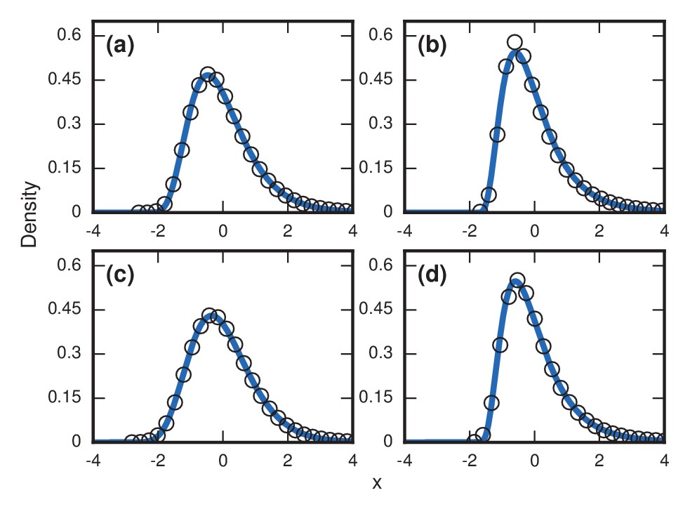
Robustness to population variability.

Simulated, fitted, and normalized distributions of incubation periods for Birth-death dynamics on a complete graph that initially has $N = 500$ nodes. Invader fitness is set at $r = 10$ . The blue curves indicate noncentral lognormals fitted via the method of moments. (a) Constant total population. (b) Growing population. At every time step, there is a constant 1/ $N$ chance that a new resident node will appear. The new node is adjacent to all preexisting nodes. (c) Shrinking population. At every time step, there is a constant 1/ $N$ chance that a random resident node will be removed. (d) Randomly varying population. At every time step, a resident node is either added or removed from the population, both events occurring with probability 1/2.

https://doi.org/10.7554/eLife.30212.014

Tables

Table 1

Model dispersion factors.

Dispersion factors (geometric standard deviations, see Box 1) for the simulated distributions of incubation periods shown in Figures 6,7,8 , for different networks and invader fitness levels $r$ . Errors represent 95% confidence intervals. Due to finite size effects, the dispersion factors exceed 1 for 1D and 2D lattices with $r = \infty$ (they should approach one as $N \to \infty$ ). Dispersion factors for the $r = 1$ case are larger than for the $r = \infty$ case, but are more uniform for different network topologies.

https://doi.org/10.7554/eLife.30212.010

Network	$r = \infty$	$r = 1$
Complete	$1.2386 \pm 0.0004$	$1.6629 \pm 0.0012$
Star	$1.3463 \pm 0.0006$	$1.6875 \pm 0.0012$
1D Lattice	$1.1418 \pm 0.0002$	$1.7907 \pm 0.0014$
2D Lattice	$1.0731 \pm 0.0003$	$1.6799 \pm 0.0012$
3D Lattice	$1.1289 \pm 0.0006$	$1.6659 \pm 0.0012$
Erdős-Rényi	$1.2586 \pm 0.0004$	$1.6900 \pm 0.0012$
Small-World	$1.2604 \pm 0.0004$	$1.7693 \pm 0.0014$
k-Regular	$1.2125 \pm 0.0003$	$1.7229 \pm 0.0013$
Scale-Free	$1.4189 \pm 0.0007$	$1.7399 \pm 0.0013$