Figures and data in Individual crop loads provide local control for collective food intake in ant colonies

Version of Record

Accepted for publication after peer review and revision.

Download
Cite
Share
CommentOpen annotations (there are currently 0 annotations on this page).

Version of Record updated: March 23, 2018 (Go to version)
Version of Record published: March 21, 2018 (This version)
Accepted Manuscript published: March 6, 2018 (Go to version)
Accepted: February 19, 2018
Received: September 3, 2017

Figures
Videos
Tables
Additional files

6 figures, 2 videos, 2 tables and 1 additional file

Figures

Figure 1 with 2 supplements

Download asset Open asset

Dynamics of food accumulation in a starved colony.

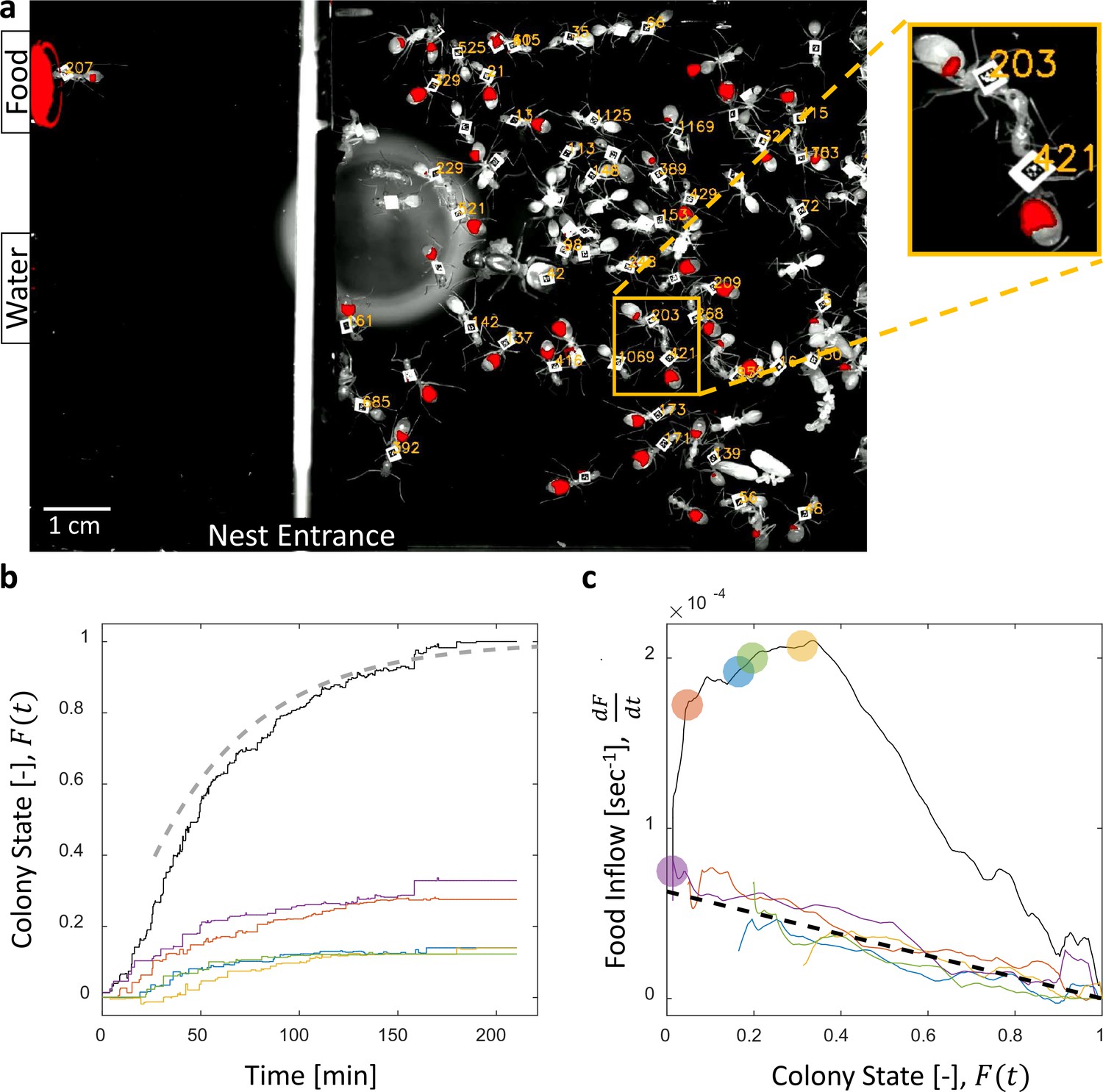
(a) A single frame from a video of a colony in the course of food accumulation. Ant identity is presented as a unique number next to her tag, and the fluorescent food is presented in red. The right side of the image is an IR-covered nest, and the left side is a neighboring open yard that includes a food source and a water source. In this frame a forager can be seen feeding from the food source (ant 207), and a trophallactic event between ants 203 and 421 is magnified. (b) Global food accumulation (normalized fluorescence), $F (t)$ , is plotted in black. The accumulated food brought by each forager, $f_{i} (t)$ is plotted in a unique color. The dashed line is the predicted colony state according to Equation 3 for $m = 0.6 \times 10^{- 4}$ , as estimated from Figure 1c. (c) The time-averaged global inflow, $\frac{d F}{d t}$ , as a function of $F (t)$ , is plotted in the black solid line. Time-averaged flows through individual foragers, $\frac{d f_{i}}{d t}$ , are plotted in unique colors (same as in panel b). Flows were calculated by differentiating the colony state and the contributions of each forager (the curves from Figure 1b) with respect to time (see Methods, Data Analysis). Colored circles on the global plot depict each forager’s first return from the food source. The black dashed line represents Equation 2, where $m$ was calculated as follows: the flow through each forager was fit with an equation of the form $\frac{d f_{i}}{d t} = m_{i} \cdot (1 - F (t))$ , and $m$ was taken to be the average of all $m_{i}$ . Results from all three experimental colonies can be found in Figure 1—figure supplements 1 and 2. Source files for panels b and c are available in Figure 1—source datas 1 and 2.

https://doi.org/10.7554/eLife.31730.003

Figure 1—source data 1 Trophallactic interactions. This data also relates to Figures 2, 3 and 6.: https://doi.org/10.7554/eLife.31730.006
Download elife-31730-fig1-data1-v2.xlsx
Figure 1—source data 2 Temporal data. This data also relates to Figures 2 and 6.: https://doi.org/10.7554/eLife.31730.007
Download elife-31730-fig1-data2-v2.xlsx

Figure 1—figure supplement 1

Download asset Open asset

Food accumulation dynamics in all three experimental colonies.

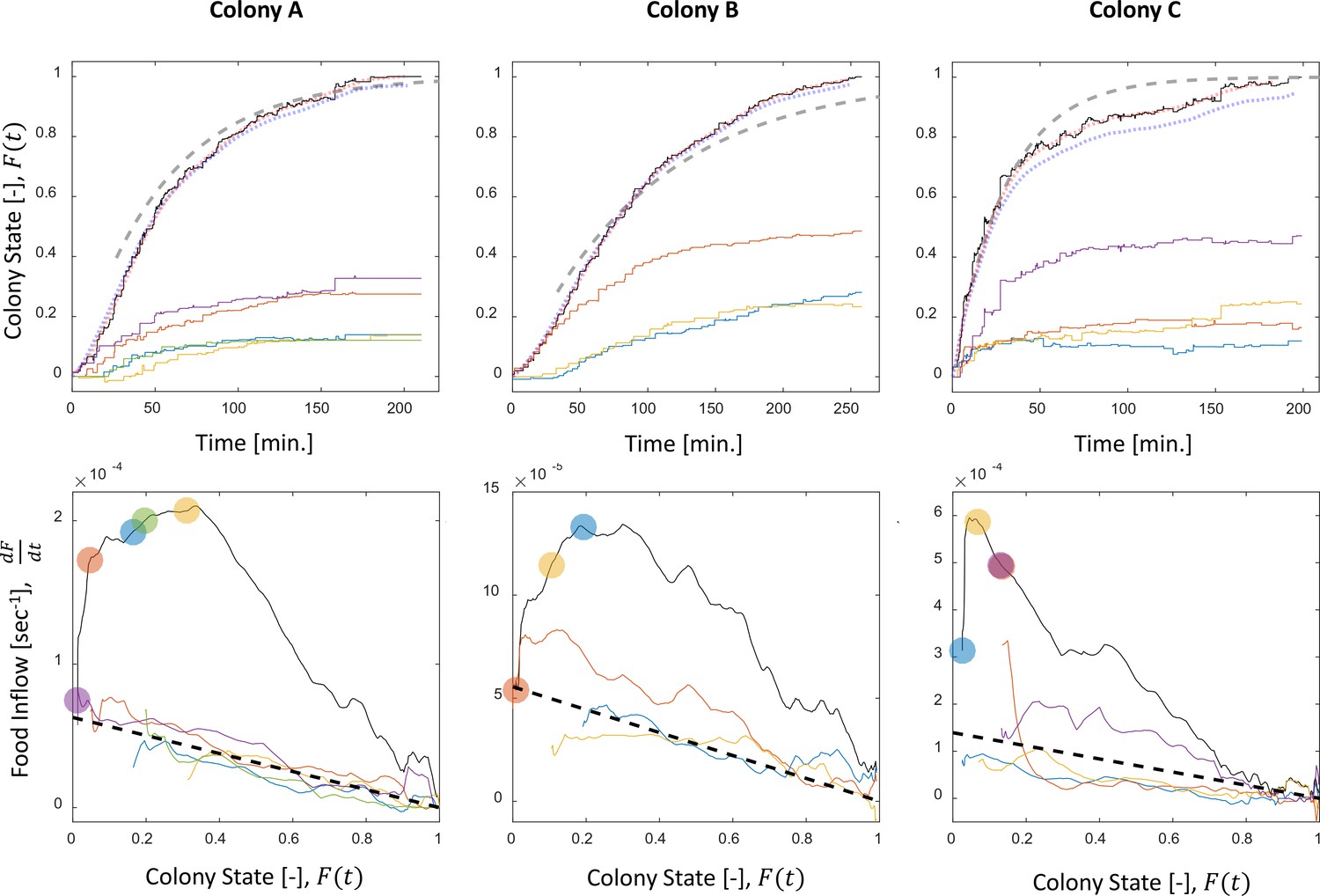
Food accumulation (top row) and food inflow (bottom row) of each experimental colony (columns). The results of Colony A are presented in Figure 1 in the main text, where a detailed explanation can be found in the caption. The smoothed data of accumulated food, which is referred to as ‘colony state’ in all other analyses, and from which the food inflow was derived (see Methods, Food flow), is presented in the red dotted curve. The blue dotted curve is the integral of the obtained food flow. This was plotted to validate the method of differentiation that was used to derive the food inflow (see Methods, Food flow).

https://doi.org/10.7554/eLife.31730.004

Figure 1—figure supplement 2

Download asset Open asset

Food flows through individual foragers and their average.

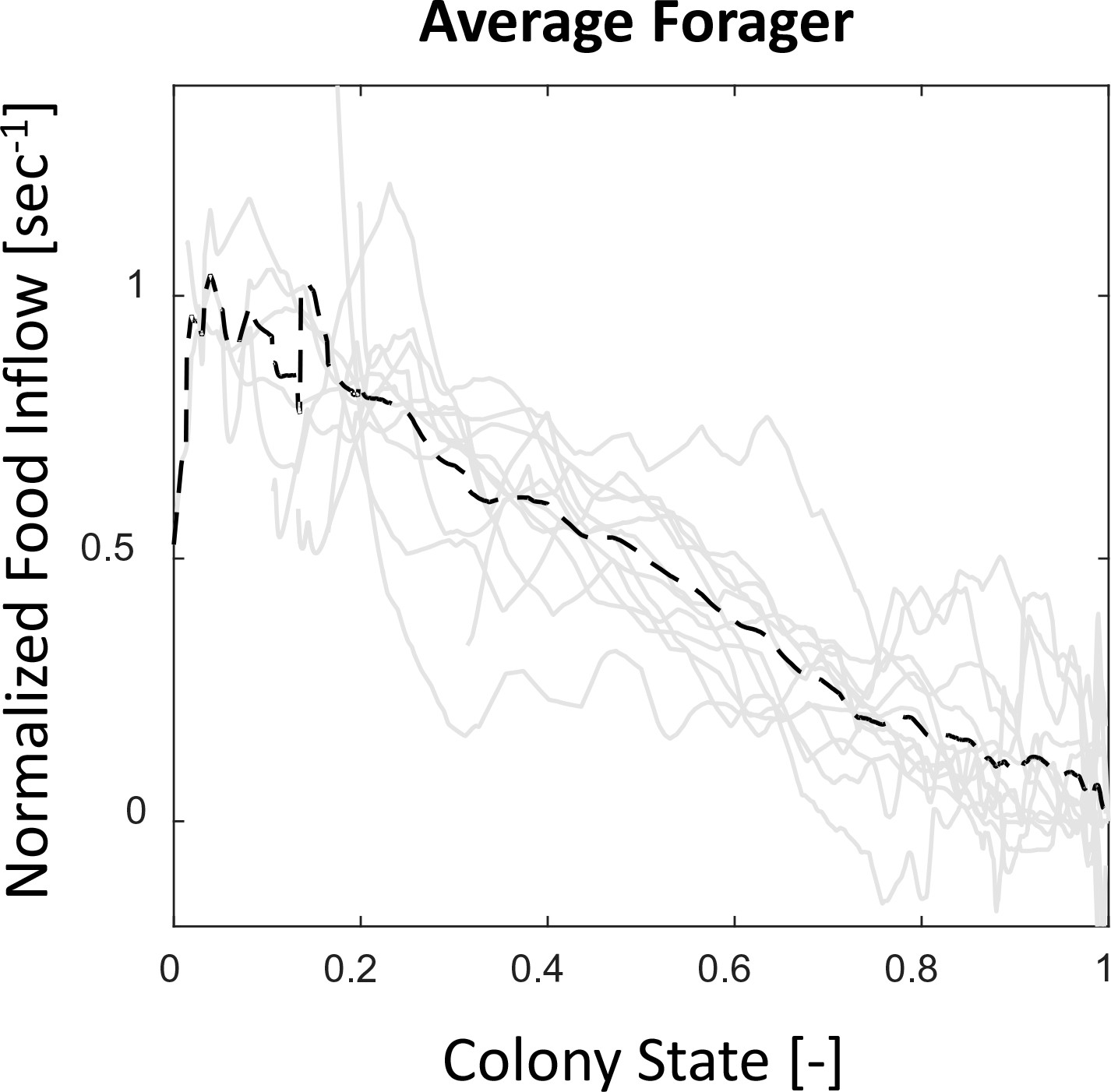
All food flows through individual foragers from all three observation experiments (gray solid lines) were normalized such that $\frac{d f_{i}}{d t} (t = 0) = 1$ , to account for scale differences between experiments. The average of all normalized flows (black dashed line) is highly linear with the colony state. Most foragers, despite starting to forage at different times, do not greatly deviate from this straight line.

https://doi.org/10.7554/eLife.31730.005

Figure 2 with 3 supplements

Download asset Open asset

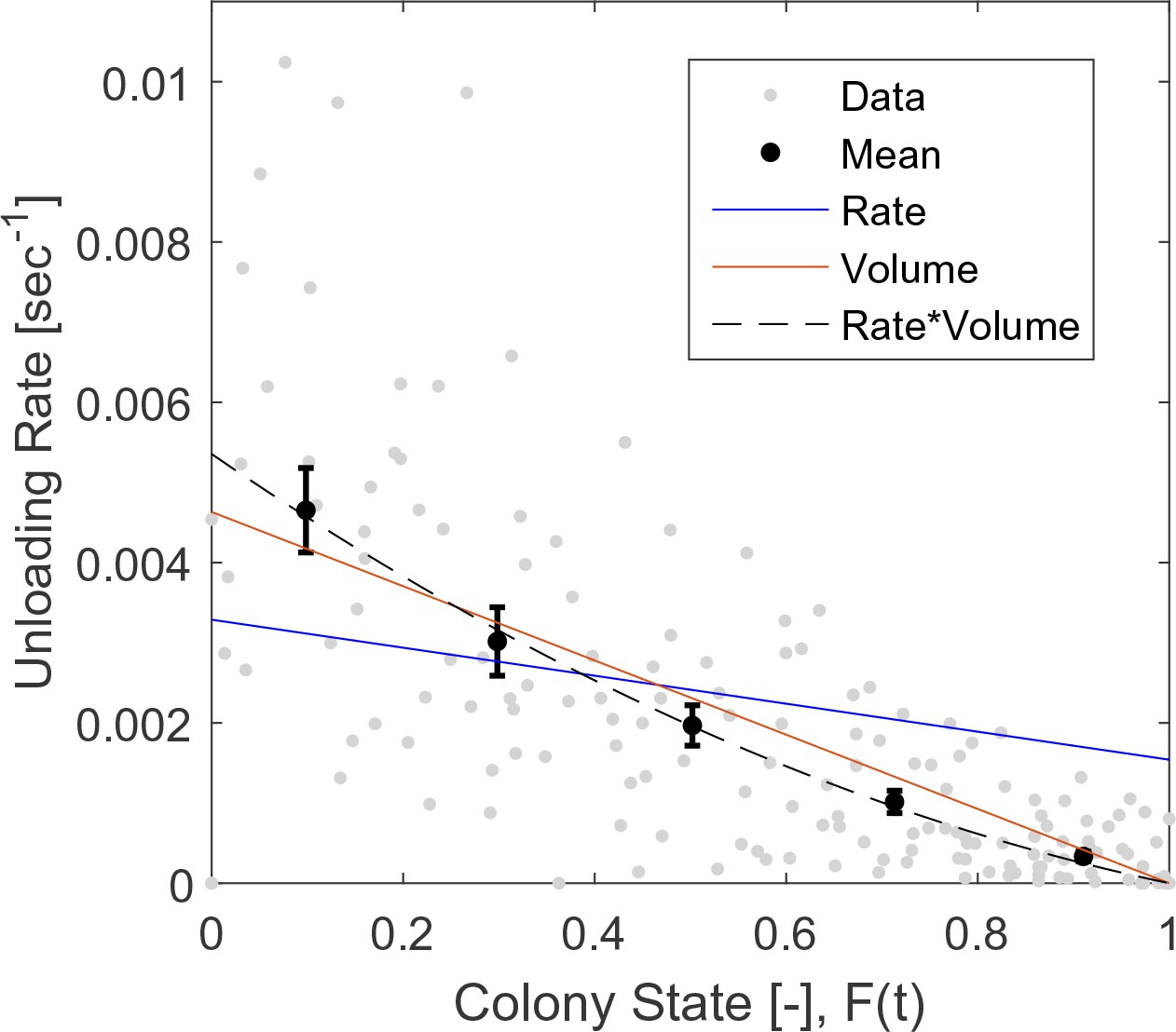
Interaction volume is the dominant component of unloading rate.

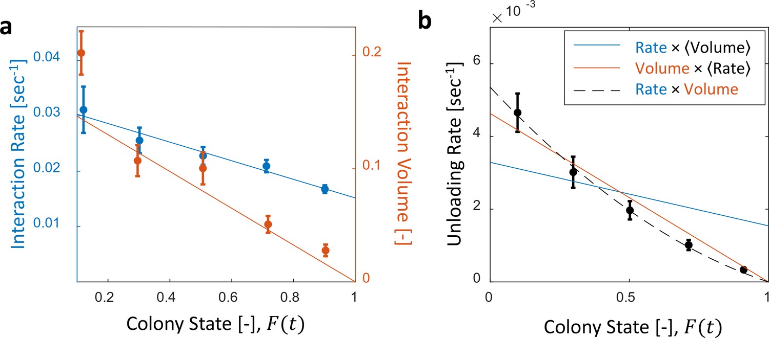
(a) Interaction rate (blue) and interaction volumes (red) both decline with increasing colony state. Binned data is presented by mean $\pm$ SEM. Interaction rate was calculated as the inverse of all intervals between interactions. The intervals were binned according to the colony state at which they occurred (n = 49, 79, 101, 170, 240 for bins 1–5, respectively. See Figure 2—figure supplement 1 for raw data and Figure 2—source data 1 for binning sensitivity analysis). Blue line depicts a linear fit $r (F) = 0.032 - 0.017 F$ , $R^{2} = 0.96$ . Interaction volumes were measured in units of pixel intensities, normalized between experiments (see Methods, Data Analysis), and binned into equally-spaced colony state bins (n = 84, 137, 165, 274, 496 for bins 1–5, respectively. See S4). Red line represents the predicted relationship between the mean interaction volume and the colony state from Equation 9, with $C_{0} = 1.14$ and $\frac{1}{λ_{0}} = 0.14$ as obtained from the fit in Figure 3a. (b) Foragers’ unloading rates at each visit in the nest were binned according to colony state (black, mean $\pm$ SEM for each bin, n = 26,26,28,39,57 for bins 1–5, respectively). Mean unloading rate values were fitted by three functions: the blue line represents a model which includes the effect of interaction rates only ( $u n l o a d i n g r a t e \propto 0.032 - 0.017 F$ , function obtained from fit in panel a, $R^{2} = 0.52$ ), the red line represents a model which includes the effect of interaction volumes only ( $u n l o a d i n g r a t e \propto 0.2 - 0.2 F$ , function obtained from fit in Figure 2—figure supplement 2, $R^{2} = 0.96$ ), and the black dashed line represents a model that incorporates the combined effects of interaction volumes and interaction rates ( $u n l o a d i n g r a t e \propto (0.032 - 0.071 F) \cdot (0.2 - 0.2 F)$ , $R^{2} = 0.99$ ). All panels in this figure represent pooled data from all three observation experiments. For raw data see Figure 2—figure supplement 3. Source file is available in Figure 1—source data 1.

https://doi.org/10.7554/eLife.31730.010

Figure 2—source data 1 Sensitivity analysis for binning interaction rate data.: https://doi.org/10.7554/eLife.31730.014
Download elife-31730-fig2-data1-v2.xlsx

Figure 2—figure supplement 1

Download asset Open asset

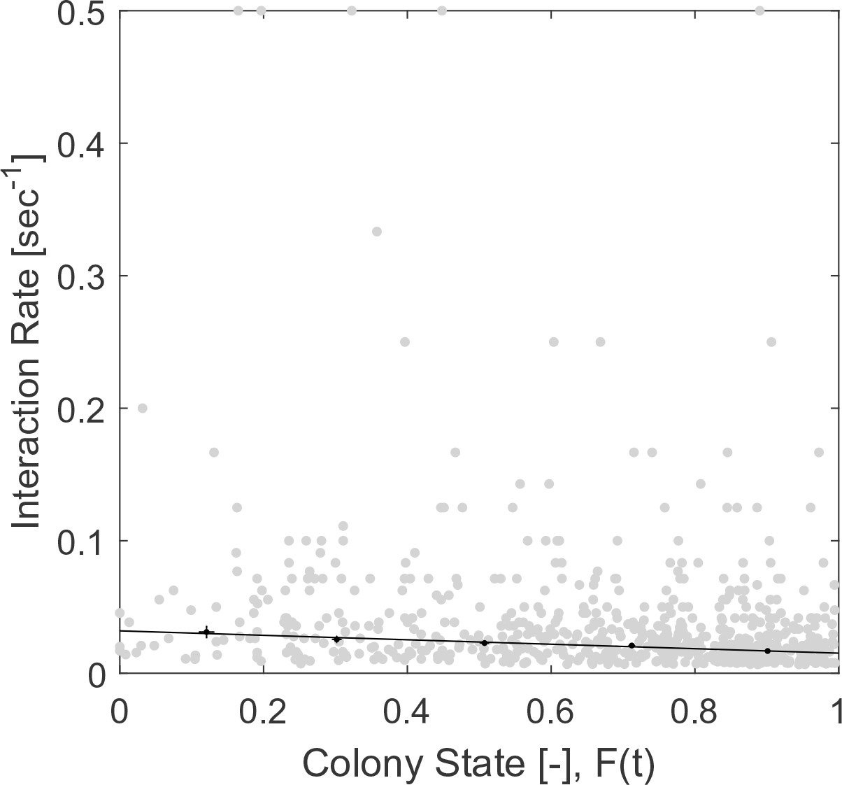
Raw (gray) and binned (black) data of interaction rates.

Each data point is the inverse of an interval between two consecutive interactions of a single forager. Binned data and linear fit are as presented in Figure 2a. The figure relates to the pooled data from all three observation experiments.

https://doi.org/10.7554/eLife.31730.011

Figure 2—figure supplement 2

Download asset Open asset

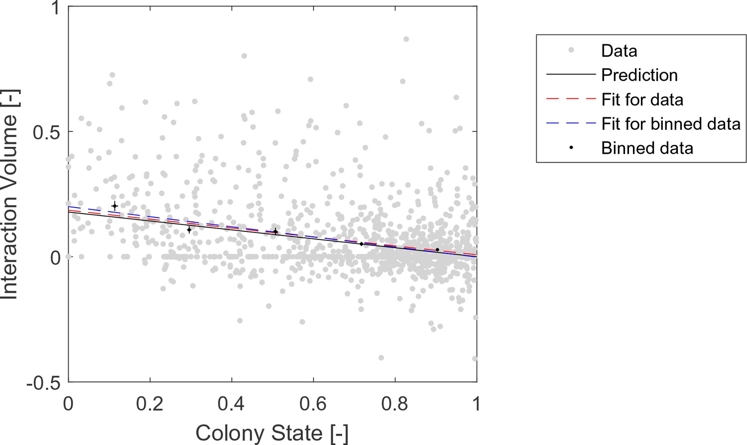
Raw data pooled from all three observation experiments (gray) and binned (black) data of interaction volumes.

Negative values represent interactions in which the forager was the receiver. Binned data and linear fit are as presented in Figure 2a. Linear fits to the raw data (red, $y = 0.185 - 0.178 x$ , $R^{2} = 0.10$ ), and to the binned data (blue, $y = 0.200 - 0.201 x$ , $R^{2} = 0.90$ ), are similar to each other and close to the prediction (black, $y = 0.163 - 0.163 x$ , $R^{2} = 0.73$ ).

https://doi.org/10.7554/eLife.31730.012

Figure 2—figure supplement 3

Download asset Open asset

Raw (gray) and binned (black) data of unloading rates.

Each data point is the unloading rate of a forager in a single visit in the nest, calculated as the amount of food she transferred in that visit (in normalized units, see Methods: Data Analysis), divided by the duration of that visit. Binned data and fits are as presented in Figure 2b. The figure relates to the pooled data from all three observation experiments.

https://doi.org/10.7554/eLife.31730.013

Figure 3 with 3 supplements

Download asset Open asset

Microscopic food flow.

(a) The distributions of interaction volumes from foragers to non-forager recipients, at seven ranges of *recipient* crop loads, follow an exponential probability density function of the form $p (v | c) = λ_{c} e^{- λ_{c} v}$ (Equation 5, Figure 3—figure supplement 1). Here the seven rate parameters of the distributions ( $λ_{c}$ ) are plotted as a function of the *recipient’s* crop load ( $c_{r e c i p i e n t}$ ). Mean $\pm$ STD of $λ_{c}$ are over different binnings of the histograms to which the exponential distribution function was fit (17 histogram binwidths uniformly covering the range [0.01–0.09]). Curve represents a fit of the function $λ_{c} = \frac{λ_{0}}{C_{0} - c}$ (Equation 6): $λ_{0} = 7.01$ , $C_{0} = 1.14$ , $R^{2} = 0.93$ . (b) Similarly to panel a, the rate parameters of the exponential distributions of interaction volumes were obtained for seven ranges of *forager* crop loads (Figure 3—figure supplement 2) and plotted as a function of the *forager’s* crop load, $c_{f o r a g e r}$ . Dashed curve represents a fit of the form $λ_{c} = \frac{c o n s t}{c_{f o r a g e r}}$ , similar to Equation 6, but instead of a fraction of the recipient’s empty crop space, $λ_{c}$ is assumed to be a fraction of the forager’s crop load. $R^{2}$ was negative, indicating that this function is no better fit to the data than a constant (solid line). (c) The distributions of ‘relative interaction volumes’, $\tilde{v}$ , wherein each interaction volume was normalized to the available space in the receiver’s crop ( $\tilde{v} = \frac{v}{C_{0} - c}$ ). The distributions collapse onto a single exponential function $p (\tilde{v}) = \frac{1}{λ} e^{- \frac{1}{λ} \tilde{v}}$ , $λ = 0.12$ , $R^{2} = 0.96$ . (d) The crop loads of non-foragers at interactions with foragers (blue, n as in b) compared to crop loads of all non-foragers in the colony (red, n = 202 per colony state bin). The distributions of crop loads at each colony state are plotted as a violin plot, and the mean $\pm$ SEM are plotted in solid lines. All panels in this figure represent pooled data from all three observation experiments. Source file is available in the Figure 1—source data 1.

https://doi.org/10.7554/eLife.31730.015

Figure 3—figure supplement 1

Download asset Open asset

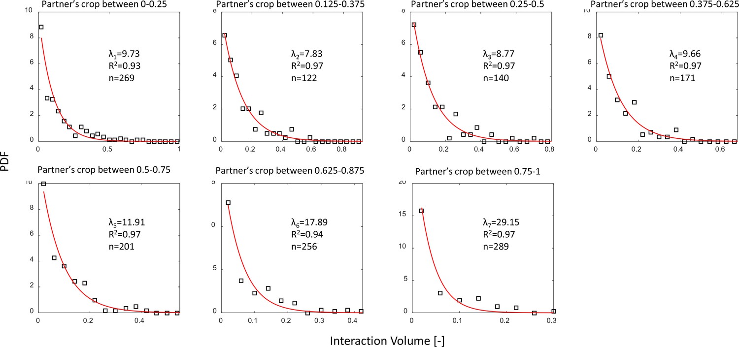
Interaction volume distributions given recipient crop load.

Each plot depicts a PDF of interaction volumes for a different range of recipient crop loads (indicated in the titles). Data was extracted from pooled data from all three observation experiments. All distributions were fit with exponentials as specified in the text (red curves). The fitted coefficients, $R^{2}$ of each fit, and sample sizes are indicated on the plots. See Methods section for details on units of food volume. To ensure that this procedure was not sensitive to histogram binwidths, it was performed on a range of binwidths as specified in the caption of Figure 3a. Here we show the results for a binwidth of 0.04.

https://doi.org/10.7554/eLife.31730.016

Figure 3—figure supplement 2

Download asset Open asset

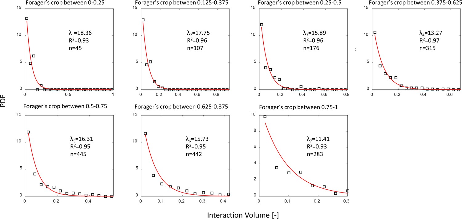
Interaction volume distributions given Forager’s crop load.

Each plot depicts a PDF of interaction volumes for a different range of forager crop loads (indicated in the titles). Data was extracted from all three observation experiments. All distributions were fit with exponentials as specified in the text (red curves). The fitted coefficients, $R^{2}$ of each fit, and sample sizes are indicated on the plots. See Methods section for details on units of food volume. To ensure that this procedure was not sensitive to histogram binwidths, it was performed on a range of binwidths as specified in the caption of Figure 3a. Here we show the results for a binwidth of 0.04.

https://doi.org/10.7554/eLife.31730.017

Figure 3—figure supplement 3

Download asset Open asset

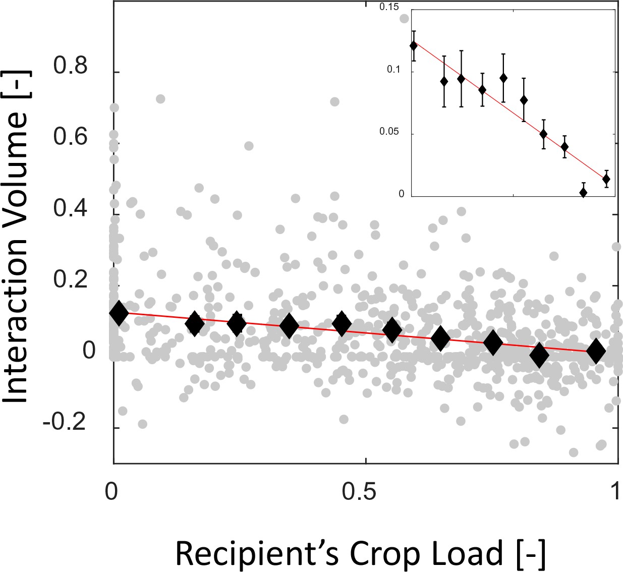
Mean interaction volumes as a function of the recipient’s crop load.

Interaction volumes (gray, pooled data from all three observation experiments) were binned according to the recipient’s crop load (black, mean $\pm$ SEM, n = 172,44,43,59,64,70,85,100,112,123 for bins 1–10, respectively) and fit with a function of the form $y = a x + b$ (red). Binned data and fit are magnified in the inset. The same fit was obtained for 5–10 bins, resulting in $a = - 0.12$ and $b = 0.13$ with $R^{2} = 0.93, 0.94, 0.94, 0.94, 0.9, 0.88$ , respectively.

https://doi.org/10.7554/eLife.31730.018

Figure 4 with 2 supplements

Download asset Open asset

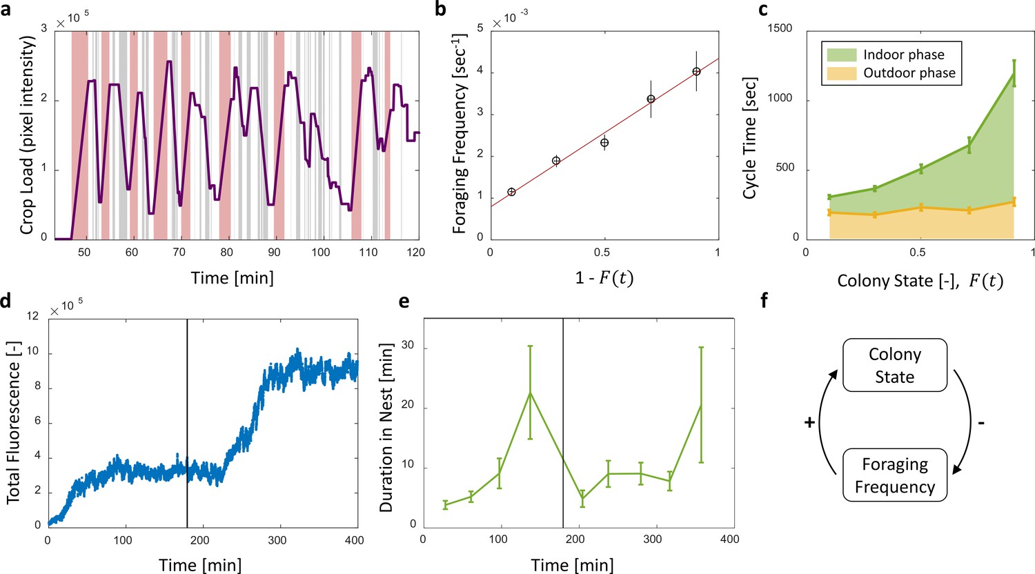
Foraging cycles.

(a) The estimated crop load of a single forager during the first two hours of an experiment. As typical for a forager, her crop load oscillates as she alternates between feeding at the food source (pink areas) and unloading in trophallaxis (gray areas) in continuous back-and-forth trips. (b) The foraging frequency of individual foragers, calculated as the inverse of cycle times (the time interval between two consecutive feeding events of a single forager), grows linearly with the empty space in the colony, $1 - F$ . Data points and error bars represent means and SEM of cycles. The pooled data from all three observation experiments is grouped into equally-spaced bins of colony state (n = 57,39,28,26,26, for bins 1–5, respectively, see Figure 4—figure supplement 1). A linear fit is presented in red: $y = {0.8 10}^{- 3} + {3.6 10}^{- 3} (1 - F)$ , $R^{2} = 0.98$ . (c) Forager cycle durations are composed of an indoor phase (green) and an outer phase (yellow), the former accounting for most of the rising trend. The pooled data from all three observation experiments was binned and averaged as in panel b (n = 26,26,28,39,57, for bins 1–5, respectively, Figure 4—figure supplement 1). (d) Food accumulation in a perturbation experiment. Food rises to an initial plateau, and rises again to a secondary plateau after new hungry ants are introduced (black line). (e) Durations of foragers in the nest in the manipulation experiment described in panel d. Durations grow longer, drop after new hungry ants are introduced (black line), and subsequently rise again. Data points and error bars represent means and standard errors of durations of cycles grouped into time bins (n = 28,36,21,14,9,28,27,19,5, for bins 1–9, respectively). Raw data and results from a second replication of the perturbation experiment are presented in Figure 4—figure supplement 2. (f) A schematic representation of the observed negative feedback between the colony state and the foraging frequency. Source file for panels b and c is available in the Figure 4—source data 1. Source file for panels d and e is available in the Figure 4—source data 2.

https://doi.org/10.7554/eLife.31730.019

Figure 4—source data 1 Foraging cycles. This data also relates to Figure 5.: https://doi.org/10.7554/eLife.31730.022
Download elife-31730-fig4-data1-v2.xlsx
Figure 4—source data 2 Manipulation experiments.: https://doi.org/10.7554/eLife.31730.023
Download elife-31730-fig4-data2-v2.xlsx

Figure 4—figure supplement 1

Download asset Open asset

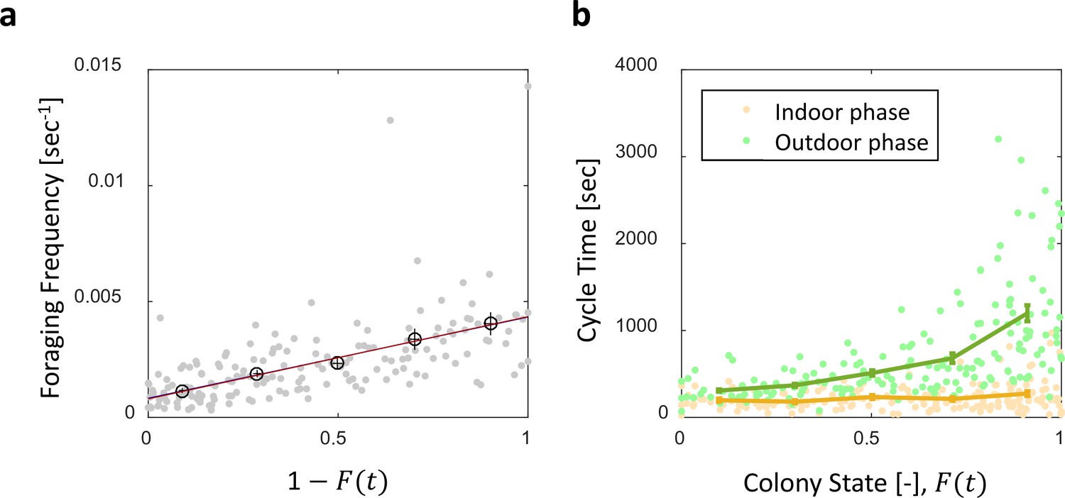
Foraging cycle times.

Both panels relate to the pooled data from all three observation experiments. (a) Foraging frequency, calculated as the inverse of cycle times (the time interval between two consecutive feeding events of a single forager) grows linearly with $1 - F$ . Raw data (gray) was binned into equally-spaced bins of colony state (n = 57,39,28,26,26, for bins 1–5, respectively, in black mean $\pm$ SEM.) Linear fits to the raw data (red) and the binned data (blue, hidden behind the red) yield similar lines: $y = {0.8 10}^{- 3} + {3.6 10}^{- 3} (1 - F)$ , $R^{2} = 0.35, 0.98$ , respectively. (b) Forager cycle durations are composed of an indoor phase (green) and an outer phase (yellow), the former accounting for most of the rising trend. Data was binned and averaged as in panel a (n = 26,26,28,39,57, for bins 1–5, respectively).

https://doi.org/10.7554/eLife.31730.020

Figure 4—figure supplement 2

Download asset Open asset

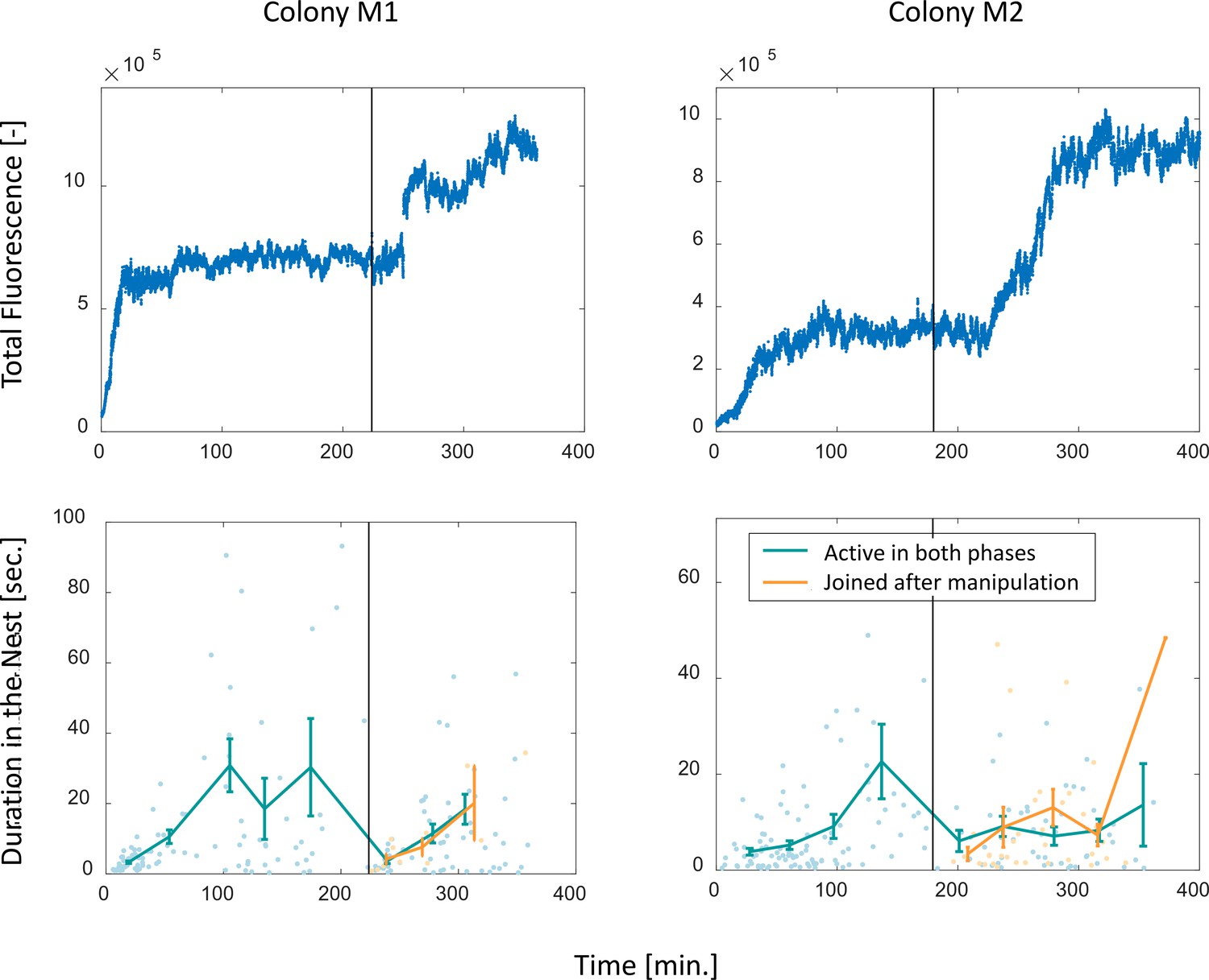
Perturbation experiments.

Food accumulation, represented by the total fluorescence (top row), and durations of foragers in the nest (bottom row), as a function of time in the two experimental colonies that underwent colony state manipulation (see Methods). Solid black line represents the time of introducing new hungry ants to the system. The results of colony M2 are presented in Figure 4d–e in the main text, where a detailed explanation may be found in the caption. Note that the plots depicting durations in the nest here differ from that in Figure 4e, in that here durations are plotted by two separate groups: those of foragers which were active during the whole experiment (M1: n = 47,13,15,13,12,16,17,14 for bins 1–8, respectively; M2: n = 28,36,21,14,5,15,18,10,4, for bins 1–9, respectively) and those of foragers that began foraging after the manipulation (M1: n = 6,3,2, for bins 1–3, respectively; M2: n = 4,13,9,9,1, for bins 1–5, respectively). In Figure 4e, all were pooled together. The observation that foragers of both groups displayed similar patterns after the manipulation highlights the causality of the effect of colony state on forager behavior as opposed to time or the forager’s history.

https://doi.org/10.7554/eLife.31730.021

Figure 5 with 1 supplement

Download asset Open asset

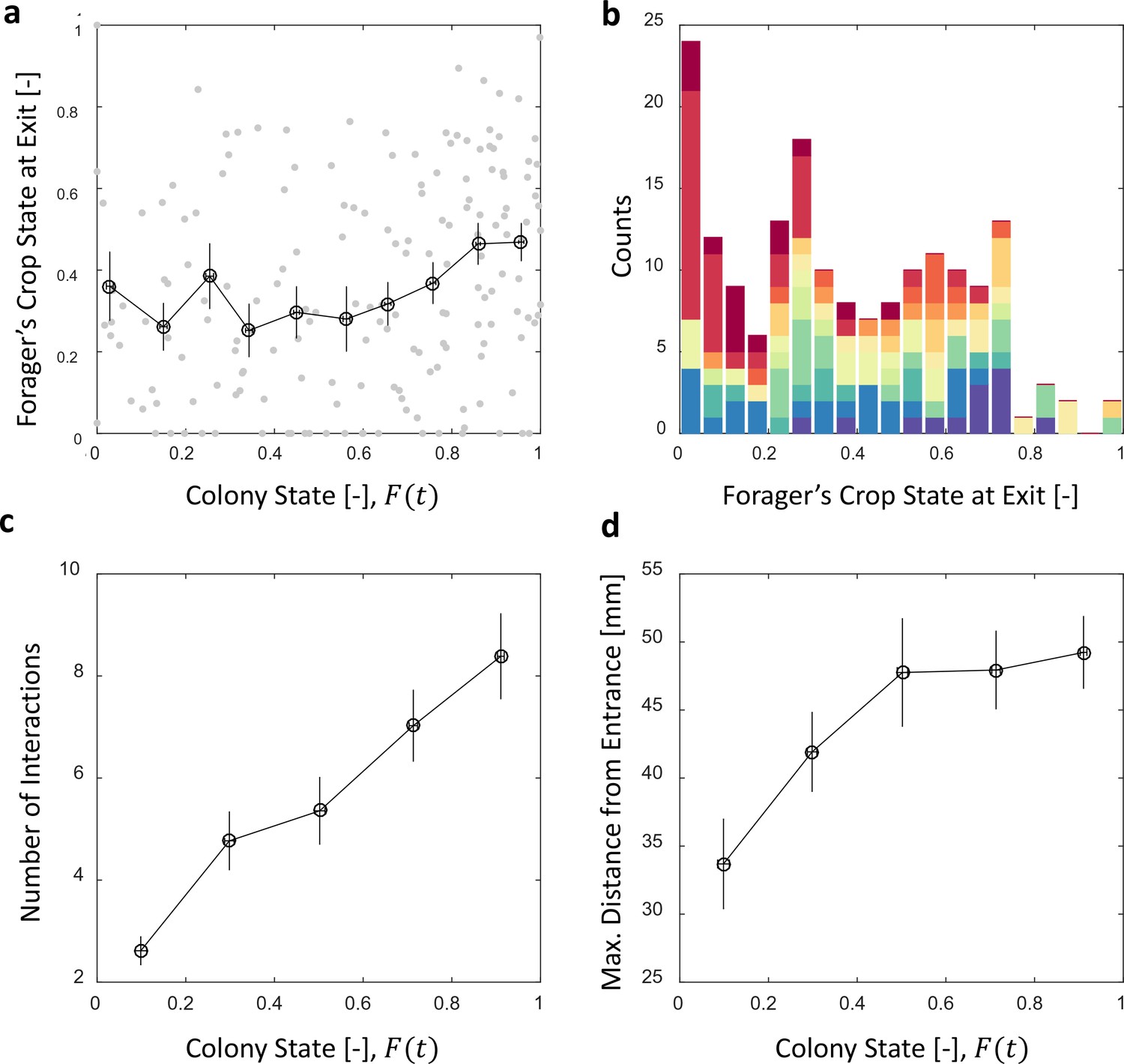
Foragers’ crop loads at exit.

(a) Foragers’ crop loads at the moments of exit were only weakly dependent on colony state (Spearman’s correlation test, $r_{s} = 0.24$ , $p = 0.001$ ), the average remaining approximately constant with only a slight rise at high colony states. Gray: raw data, black: mean $\pm$ SEM of binned data (n = 11,15,13,13,15,13,17,22,27,30 for bins 1–10, respectively). (b) The wide distribution of foragers’ crop loads at the moments of exit (n = 176). Each color represents a different forager, revealing that the distribution of crop loads upon exit is wide within each forager and not due to inter-individual variability. (c) The number of interactions a forager has in a single visit to the nest rises as the colony satiates, mean $\pm$ SEM of binned data (n = 26,26,28,39,57 for bins 1–5, respectively, Figure 5—figure supplement 1a). (d) Foragers reach deeper locations in the nest as the colony satiates, mean $\pm$ SEM of binned data (n as in panel c, Figure 5—figure supplement 1b). All panels relate to the pooled data from all three observation experiments. Source file is available in the Figure 4—source data 1.

https://doi.org/10.7554/eLife.31730.024

Figure 5—figure supplement 1

Download asset Open asset

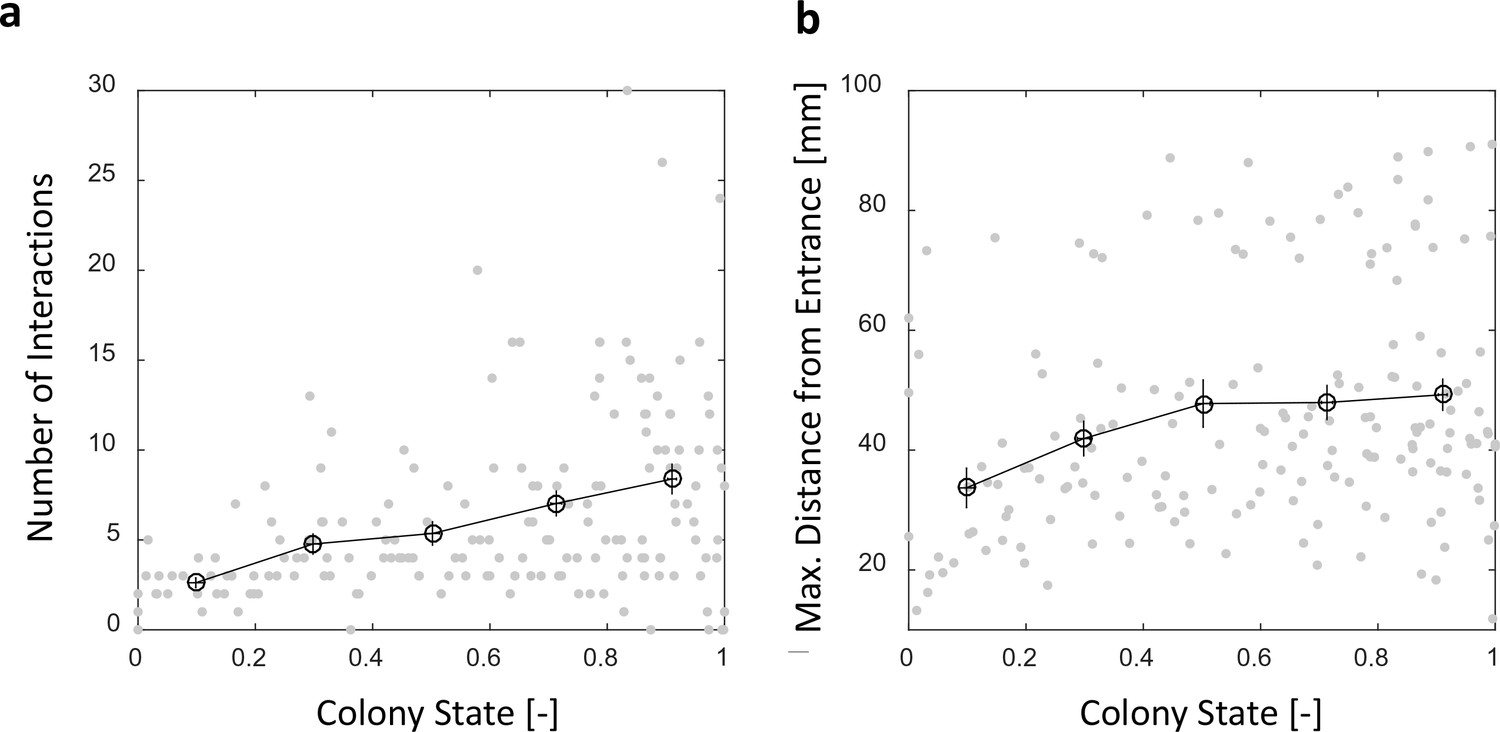
Number of interactions and maximal distance from entrance in a forager’s visit in the nest.

Both panels relate to the pooled data from all three observation experiments. (a) The number of interactions in which a forager participates in a single visit to the nest rises as the colony satiates. Raw data (gray) and mean $\pm$ SEM of binned data (black, n = 26,26,28,39,57 for bins 1–5, respectively). (b) Foragers reach deeper locations in the nest as the colony satiates. Raw data (gray) and mean $\pm$ SEM of binned data (Black, n as in panel c). Data seems separated into clusters (upper and lower clouds) due to differences in the location of most of the ants within the nest between experiments.

https://doi.org/10.7554/eLife.31730.025

Figure 6

Download asset Open asset

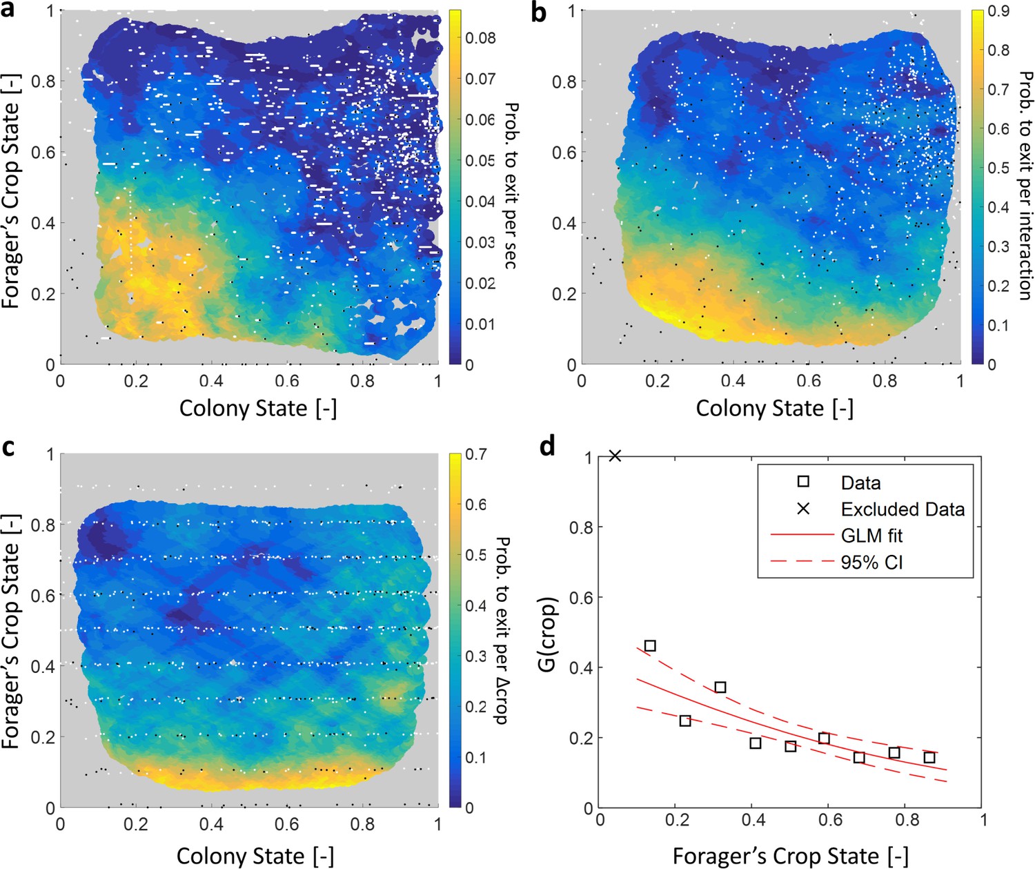
Forager exits.

(**a–c**) Forager exit probabilities as a function of the colony state and her own crop state. All panels relate to the pooled data from all three observation experiments. Observations are plotted on a 2-dimensional space of the forager’s crop state and the colony state, as black and white dots (white - ‘stay’ observations, black - ‘exits’). An observation was classified as an ‘exit’ if the forager left the nest before the next considered observation. The colored surface represents the estimated local probability to exit on this space, calculated as the fraction of ‘exits’ out of all observations in each bin in the space: the color of each pixel on the surface represents the probability calculated based on the $n$ closest data points, and the pixel’s location is the average location of these points (a: $n = 300$ , b-c: $n = 30$ ). The three panels consider three possible decision rates: Constant decision rate (a) where all observations, taken every two seconds, were considered to be decision points (excluding observations during trophallaxis). Decision rate matched to interaction rate (b) where only observations at ends of interactions were considered to be decision points. Decision rate matched to unloading rate (c) where only observations taken each time a forager unloaded $Δ c r o p$ food, were considered to be decision points ( $Δ c r o p$ =10% of the forager’s capacity). (d) $G (c r o p)$ , a projection of the two-dimensional probability presented in panel c on the forager’s crop state axis. Since foragers’ crop loads rarely rose in the nest, their lowest crop observation in a visit was generally an ‘exit’, so the calculated probability to exit in the lowest crop interval was 1. To ensure that the crop state played a role beyond this extreme effect, the GLM fit did not include the lowest crop interval. The crop load effect was significant: $β_{c} = - 1.93$ , $p < 0.001$ . Source file for panels a and c is available in the Figure 1—source data 2. Source file for panel b is available in the Figure 1—source data 1.

https://doi.org/10.7554/eLife.31730.026

Videos

Video 1

Download asset

posterframe for video — A trophallactic event.

Two *Camponotus sanctus* ants engaged in trophallaxis of fluorescent liquid food (presented in purple).

https://doi.org/10.7554/eLife.31730.008

Video 2

Download asset

Tables

Table 1

Logistic fits for a forager’s probability to exit ( $P$ ) as a function of her crop load and the colony state.

A two-dimensional logistic function of the form $P = {(1 + e^{- (α + β \cdot c r o p + γ \cdot c o l o n y)})}^{- 1}$ was fit to each estimated probability to exit from Figure 6a–c. The effect of each factor is reflected in its fitted coefficient. Within each model, effects can be compared to one another because the values of $c r o p$ and $c o l o n y$ lay on the same scale between 0 and 1. In the constant decision rate model, all coefficients were comparable in value, indicating that $c r o p$ and $c o l o n y$ had similar meaningful effects on the probability to exit. In the model where decision rate was matched to interaction rate, the effect of $c o l o n y$ was weaker than the effect of $c r o p$ , but both were still meaningful. In the model where decision rate was matched to unloading rate, the effect of $c o l o n y$ approached 0 and was very weak compared to the effect of $c r o p$ .

https://doi.org/10.7554/eLife.31730.027

Decision rate model	Factor	Coefficient	95% CI		$R^{2}$
Constant	Intercept	$α = - 1.914$	$- 1.921$	$- 1.906$	$0.81$
	Colony State	$β = - 1.763$	$- 1.778$	$- 1.747$
	Forager’s Crop	$γ = - 2.330$	$- 2.347$	$- 2.312$
Interaction Rate	Intercept	$α = 2.701$	$2.686$	$2.716$	$0.92$
	Colony State	$β = - 2.199$	$- 2.218$	$- 2.181$
	Forager’s Crop	$γ = - 5.810$	$- 5.837$	$- 5.783$
Unloading Rate	Intercept	$α = - 0.093$	$- 0.105$	$- 0.081$	$0.71$
	Colony State	$β = 0.499$	$0.482$	$0.515$
	Forager’s Crop	$γ = - 3.092$	$- 3.115$	$- 3.069$